Download
1 / 44
450 likes | 567 Views
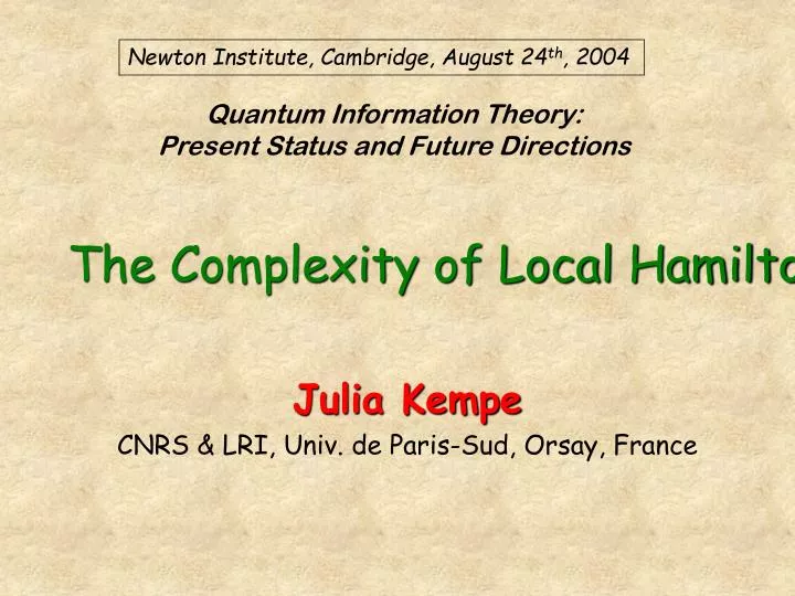
Newton Institute, Cambridge, August 24 th , 2004. Quantum Information Theory: Present Status and Future Directions. The Complexity of Local Hamiltonians. Julia Kempe CNRS & LRI, Univ. de Paris-Sud, Orsay, France. Also implies:.

E N D
Newton Institute, Cambridge, August 24th, 2004 Quantum Information Theory: Present Status and Future Directions The Complexity of Local Hamiltonians Julia Kempe CNRS & LRI, Univ. de Paris-Sud, Orsay, France
Also implies: 2-local adiabatic computation is equivalent to standard quantum computation Joint work with Oded Regev and Alexei Kitaev • Result: • 2-local Hamiltonian is QMA complete J. K., Alexei Kitaev and Oded Regev, quant-ph/0406180
Outline • A Bit of History • QMA • Local Hamiltonians • Previous Constructions • The 3-qubit Gadget • Implications • Adiabatic computation • Other applications of the technique
Complexity Theory: • classify “easy” and “hard” A Bit of (ancient) History
“yes” instance: x L V 1 (accept) witness: y “no” instance: x L V 0 (reject) for all “witnesses” y A Bit of (ancient) History • NP – Nondeterministic Polynomial Time: • Def. L NP if there is a poly-time verifier V and • a polynomial p s.t.
0 - false 1 - true 0 = 1, 1 = 0 0 1 1 0 0 0 1 1 “yes” instance: SAT V= (y) 1 (true, accept) witness: y=011000… “no” instance: SAT V= (y) 0 (false, reject) for all “witnesses” y=010110… Example: SAT Formula: • SAT iff there is a satisfying assignment for x1,…,xn (i.e. all clauses true simultaneously).
SAT L L SAT 1 0 1 x y y y=011000… y=010110… V 0 NP complete A languageis NP complete if it is in NP and as hard as any other problem in NP. Cook-Levin Theorem: SAT is NP-complete NP NP-complete x
MAX2SAT is NP-complete MAX2SAT: Input: Formula with 2 variables per clause, number m Output:1(accept) if there is an assignment that violates m clauses 0(reject) all assignments violate >m clauses NP complete 3SAT: 3 variables per clause 3 variables Cook-Levin Theorem: 3SAT is NP-complete 2SAT is in P (there is a poly time algorithm).
witness: | prob 0 (reject) for all “witnesses” | prob 1 (accept) “yes” instance: x Lyes V • QMA – Quantum Merlin Artur = BQNP = “Quantum NP” • Def. L QMA if there is a poly-time quantum verifier V and • a polynomial p s.t. “no” instance: x Lno V QMA 1 (accept) prob 1- 0 (reject) prob 1-
More recent (quantum) History • QMA – Quantum Merlin Artur = BQNP • Def. L QMA if there is a poly-time quantum verifier V and • a polynomial p s.th. • First studied in [Knill’96] and [Kitaev’99] – called it BQNP • “QMA” coined by [Watrous’00] – also: group-nonmembership QMA Kitaev’s quantum Cook-Levin Theorem (’99): Local Hamiltonian is QMA-complete.
Local Hamiltonians • Def. k-local Hamiltonian problem: • Input: k-local Hamiltonian , , Hi acts on k • qubits, a<b constants • Promise: • smallest eigenvalue of H either a or b (b-a const.) • Output: • 1 if H has eigenvalue a • 0 if all eigenvalues of H b
Intuition: Formula: , Hamiltonians: H2 local Hamiltonians H1 Satisfying assignment is groundstate of • Energy-penalty 1 for each unsatisfied constraint. • x1x2 … xn| H |x1x2 … xn = #unsatisfied constraints Local Hamiltonians Penalties for: x1x2x3 = 010 x3x4x5 = 100 …
NP and QMA QMA-completeness? NP-completeness: Verifier V: x1 x2 … y1 y2 … 0 0 … x input 1 witness y … ancilla 0
Verifier Ux : | |0 |0 … |1 H C C H ancilla qubits … • input ? • propagation ancilla |0|1 … |T • output No local way to check! NP and QMA QMA-completeness? NP-completeness: Verifier Vx : y1 y2 … 0 0 … y 1 witness … ancilla 0 3-clauses check: z01 z02 … z03 z04 … zTN z0N z1N z2N t = 0 1 2 3 4 … T
NP and QMA QMA-completeness? NP-completeness: Verifier Vx : Verifier Ux : | |0 |0 … y1 y2 … 0 0 … |1 H C y 1 witness C H … ancilla qubits … ancilla 0 3-clauses check: ||0=|0|1 … |T • input + ? + + + • propagation • output |0 |1 |2 |T | |0|0+|1|1+…+|T|T witness = sum over history
but: • MAX2SAT is NP-complete • 2-local Hamiltonian is NP-hard More recent (quantum) History QMA-completeness: NP-completeness: • log|x|-local Hamiltonian is QMA-compl. • [Kitaev’99] • 5-local Hamiltonian is QMA-compl. • [Kitaev’99] • 3-local Hamiltonian is QMA-compl. • [KempeRegev’02] • 3SAT is NP-complete • 2SAT is in P 2-local Hamiltonian???? Is 2-local Hamiltonian QMA-complete?? • 1-local Hamiltonian is in P
Outline • A Bit of History • QMA • Local Hamiltonians • Previous Constructions • The 3-qubit Gadget • Implications • Adiabatic computation • Other applications of the technique
input Time register {|0, |1,…, |T} Computation qubits • propagation • output Kitaev’s log-local Construction Verifier Ux : |1 | witness = sum over history m N-m T T=poly(N) Local Hamiltonians check: H= Jin Hin + Jprop Hprop + Hout
Kitaev’s log-local Construction Verifier: Ux=UTUT-1…U1 H= Jin Hin + Jprop Hprop + Hout To show: If Ux accepts with prob. 1- on input |,0, then H has eigenvalue . If Ux accepts with prob. on all |,0, then all eigenvalues of H ½-.
|Hprop| =0 |Hout| Completeness Verifier: Ux=UTUT-1…U1 H= Jin Hin + Jprop Hprop + Hout To show: If Ux accepts with prob. 1- on input |,0, then H has eigenvalue . If Ux accepts with prob. on all |,0, then all eigenvalues of H ½-. |Hin| =0
Idea (Kitaev): unary |t | 11…100…0 t T-t |tt| |1010|t,t+1 |tt-1| |110100|t-1,t,t+1 Penalise illegal time states: Sclock - space of legal time-states is preserved (invariant) 5-local Hamiltonians Log-local terms:
Give a high energy penalty to illegal time states to effectively prevent transitions outside Sclock : (|10|t)|Sclock = |tt-1| 3-local Hamiltonians |tt-1| |110100|t-1,t,t+1 5-local terms: Idea [KR’02]: |110100|t-1,t,t+1 |10|t H Sclock
Outline • A Bit of History • QMA • Local Hamiltonians • Previous Constructions • The 3-qubit Gadget • Implications • Adiabatic computation • Other applications of the technique
… Spectrum: H H’ = H + V Energy gap: ||H||>>||V|| 0 groundspace S Three-qubit gadget Idea: use perturbation theory to obtain effective 3-local Hamiltonians from 2-local ones by restricting to subspaces What is the effective Hamiltonian in the lower part of the spectrum?
Case 1: Energy gap>>> ||V|| V--- restriction of V to S V++ - restriction of V to S S S Perturbation Theory Spectrum: H H’ = H + V S Energy gap: ||H||>>||V|| 0 groundspace S What is the effective Hamiltonian in the lower part of the spectrum? Projection Lemma: Heff = V-- (same spectrum) =O(||V||2/)
Case 2: Fine tune the energy gap> ||V|| V--- restriction of V to S V++ - restriction of V to S S S Theorem: Perturbation Theory Spectrum: H H’ = H + V S Energy gap: ||H||>>||V|| 0 groundspace S What is the effective Hamiltonian in the lower part of the spectrum?
First order Third order Second order Perturbation Theory Theorem: H S Energy gap: 0 groundspace S H’ = H + V The lower spectrum of H’ is close to the spectrum of Heff (under certain conditions).
Projection Lemma Perturbation Theory Theorem: First order: ||V||2 << H S Energy gap: 0 groundspace S H’ = H + V The lower eigenvalues (<||V||) of H’ are close to the eigenvalues of Heff (under certain conditions).
2 2 3 3 P2XB P3XC ZZ B C ZZ ZZ A P1XA 1 1 Terms in H’ are 2-local H=P1P2P3 3-local Heff=P1P2P3 3-local Three-qubit gadget
ZZ B C S={|001,|010,|100, |110,|101,|011} =-3 ZZ ZZ Energy gap: A S={|000, |111} 0 Three-qubit gadget H’ = H + V
S V-+ V+- V++ Second order: S S S S V-+ V+- V-- First order: S S Third order: S S Theorem: Three-qubit gadget H’ = H + V 2 3 P2XB P3XC B C S={|001,|010,|100, |110,|101,|011} =-3 Energy gap: A P1XA S={|000, |111} 0 1
|100 Ex.: P1XA P1XA |000 |000 Three-qubit gadget 2 3 P2XB P3XC B C S={|001,|010,|100, |110,|101,|011} =-3 Energy gap: A P1XA S={|000, |111} 0 1 S V-+ V+- Second order: S S Theorem:
P2XB |100 |110 Ex.: P1XA P3XC |000 |111 Three-qubit gadget H’ = H + V 2 3 P2XB P3XC B C S={|001,|010,|100, |110,|101,|011} =-3 Energy gap: A P1XA S={|000, |111} 0 1 V++ S S V-+ V+- Third order: S S Theorem:
Three-qubit gadget 2 3 P2XB P3XC H’ = H + V B C A P1XA 1 Theorem:
Three-qubit gadget 2 3 P2XB P3XC H’ = H + V B C A P1XA 1 Theorem:
Three-qubit gadget 2 3 P2XB P3XC H’ = H + V B C A P1XA 1 Theorem:
H V =-3 -1 Heff 0 0 const. Three-qubit gadget 2 3 P2XB P3XC H’ = H + V B C A P1XA 1 Theorem:
2-local Hamiltonian is QMA-complete • start with the QMA-complete 3-local Hamiltonian • replace each 3-local term by 3-qubit gadget
Outline • A Bit of History • QMA • Local Hamiltonians • Previous Constructions • The 3-qubit Gadget • Implications • Adiabatic computation • Other applications of the technique
Standard quantum circuit: |0…0 |T Adiabatic simulation*: T gates • Hfinal • groundstate • Hinitial • groundstate • |0…0 |0 T’=poly(T): If gap 0(H(t))-1(H(t)) between groundstate and first excited state is 1/poly(T) H(t) = (1-t/T’)Hinitial +t/T’ Hfinal *D. Aharonov, W. van Dam, J. Kempe, Z. Landau, S. Lloyd, O. Regev: "Adiabatic Quantum Computation is Equivalent to Standard Quantum Computation", lanl-report quant-ph/0405098 Implications for Adiabatic Computation • Adiabatic computation [Farhi et al.’00]: • “track” the groundstate of a slowly varying Hamiltonian
adiabat |0…0 |0 Log-local*: H(t) = (1-t/T’) Hin + t/T’ Hprop *D. Aharonov, W. van Dam, J. Kempe, Z. Landau, S. Lloyd, O. Regev: "Adiabatic Quantum Computation is Equivalent to Standard Quantum Computation", lanl-report quant-ph/0405098 Implications for Adiabatic Computation Our result also implies: 2-local adiabatic computation is equivalent to standard quantum computation Replace with 2-local: H(t) = (1-t/T’)(Hin+Jclock Hclock) + t/T’(Hpropgadget+Jclock Hclock)
-2ZA -1P1XA -1P2XA H=P1P2 Heff=P1P2 “Proxy Interaction”: (with A. Landahl) -1Z1ZA -1X2XB -2YAYB Heff=Z1X2 Other applications of the gadget(work in progress) “Interaction at a distance”: H=Z1X2 only XX,YY,ZZ available Useful for Hamiltonian-based quantum architectures
References Quantum Complexity : J. Kempe, A. Kitaev, O. Regev: “The Complexity of the local Hamiltonian Problem”, quant-ph/0406180, to appear in Proc. FSTTCS’04 J. Kempe and O. Regev: "3-Local Hamiltonian is QMA-complete",Quantum Information and Computation, Vol. 3 (3), p.258-64 (2003), lanl-report quant-ph/0302079 Adiabatic Computation : D. Aharonov, W. van Dam, J. Kempe, Z. Landau, S. Lloyd, O. Regev: "Adiabatic Quantum Computationis Equivalent to Standard Quantum Computation", lanl-report quant-ph/0405098, to appear in FOCS’04 *Photo: Oded Regev: Ladybug reading “3-local Hamiltonian” paper
prob 1- prob 0 (reject) prob 1- prob 1 (accept) “yes” instance: x Lyes V MA – Merlin-Artur: Def. L MA if there is a poly-time verifier V and a polynomial p s.t. “no” instance: x Lno V MA 1 (accept) witness: y 0 (reject) for all “witnesses” y