Download
1 / 25
1.33k likes | 4.46k Views
Modern Portfolio Theory and the Markowitz Model. Alex Carr Nonlinear Programming. Louis Bachelier. Father of Financial Mathematics The Theory of Speculation , 1900 The first to model the stochastic process, Brownian Motion Stock options act as elementary particles. John Burr Williams.

E N D
Modern Portfolio Theory and the Markowitz Model Alex Carr Nonlinear Programming
Louis Bachelier • Father of Financial Mathematics • The Theory of Speculation, 1900 • The first to model the stochastic process, Brownian Motion • Stock options act as elementary particles
John Burr Williams • Theory of Investment Value, 1938 • Present Value Model • Discounted Cash Flow and Dividend based Valuation • Assets have an intrinsic value • Present value of it’s future net cash flows • Dividend distributions and selling price
Harry Markowitz • Mathematics and Economics at University of Chicago • Earlier Models Lacked Analysis of Risk • Portfolio Selection in the Journal of Finance, 1952 • Primary theory of portfolio allocation under uncertainty • Portfolio Selection: Efficient Diversification of Investments, 1959 • Nobel Prize • Markowitz Efficient Frontier and Portfolio
Foundations • Expected return of an asset is the mean • Risk of an asset is the variability of an asset’s historical returns • Reduce the risk of an individual asset by diversifying the portfolio • Select a portfolio of various investments • Maximize expected return at fixed level of risk • Minimize risk at a fixed amount of expected return • Choosing the right combination of stocks
Model Assumptions • Risk of a portfolio is based on the variability of returns from the said portfolio. • An investor is risk averse. • An investor prefers to increase consumption. • The investor's utility function is concave and increasing.
Model Assumptions • Analysis is based on single period model of investment. • An investor either maximizes his portfolio return for a given level of risk or maximum return for minimum risk. • An investor is rational in nature.
Risk • Standard deviation of the mean (or return) • Systematic Risk: market risks that cannot be diversified away • Interest rates, recessions and wars • Unsystematic Risk: specific to individual stocks and can be diversified away • Not correlated with general market moves
Diversification • Optimal: 25-30 stocks • Smooth out unsystematic risk • Less risk than any individual asset • Assets that are not perfectly positively correlated • Foreign and Domestic Investments • Mutual Funds
Correlation Negative Positive • None −0.09 to 0.0 0.0 to 0.09 • Small −0.3 to −0.1 0.1 to 0.3 • Medium −0.5 to −0.3 0.3 to 0.5 • Strong −1.0 to −0.5 0.5 to 1.0
Expected Return • Individual Asset • Weighted average of historical returns of that asset • Portfolio • Proportion-weighted sum of the comprising asset’s returns
The Process • First: • Determine a set of Efficient Portfolios • Second: • Select best portfolio from the Efficient Frontier
Risk and Return • Either expected return or risk will be the fixed variables • From this the other variable can be determined • Risk, standard deviation, is on the Horizontal axis • Expected return, mean, is on the Vertical axis • Both are percentages
Plotting the Graph • All possible combinations of the assets form a region on the graph • Left Boundary forms a hyperbola • This region is called the Markowitz Bullet
Determining the Efficient Frontier • The left boundary makes up the set of most efficient portfolios • The half of the hyperbola with positive slope makes up the efficient frontier • The bottom half is inefficient
Indifference Curve • Each curve represents a certain level of satisfaction • Points on curve are all combinations of risk and return that correspond to that level of satisfaction • Investors are indifferent about points on the same curve • Each curve to the left represents higher satisfaction
Optimal Portfolio • The optimal portfolio is found at the point of tangency of the efficient frontier with the indifference curve • This point marks the highest level of satisfaction the investor can obtain • The point will be different for every investor because indifference curves are different for every investor
Capital Market Line • E(RP)= IRF + (RM - IRF)σP/σM • Slope = (RM – IRF)/σM • Tangent line from intercept point on efficient frontier to point where expected return equals risk-free rate of return • Risk-return trade off in the Capital Market • Shows combinations of different proportions of risk-free assets and efficient portfolios
Additional Use of Risk-Free Assets • Invest in Market Portfolio • But CML provides greatest utility • Two more choices: • Borrow Funds at risk-free rate to invest more in Market Portfolio • Combinations to the right of the Market Portfolio on the CML • Lend at the risk-free rate of interest • Combinations to the left of the Market Portfolio on the CML
Criticisms • There are a very large number of possible portfolio combinations that can be made • Lots of data needs to be included • Covariances • Variance • Standard Deviations • Expected Returns • Asset returns are, in reality, not normally distributed • Large swings occur much more often • 3 to 6 standard deviations from the mean
Criticisms • Investors are not “rational” • Herd Behavior • Gamblers • Fractional shares of assets cannot usually be bought • Investors have a credit limit • Cannot usually buy an unlimited amount of risk-free assets