Download
1 / 81
810 likes | 1.17k Views
CPSC-608 Database Systems. Fall 2010. Instructor: Jianer Chen Office: HRBB 315C Phone: 845-4259 Email: chen@cse.tamu.edu. Notes #4. SQL: Structured Query language. How does SQL manipulate (read/write) tables? (continued). in tables (relations). database administrator. lock table.

E N D
CPSC-608 Database Systems Fall 2010 Instructor: Jianer Chen Office: HRBB 315C Phone: 845-4259 Email: chen@cse.tamu.edu Notes #4
SQL: Structured Query language How does SQL manipulate (read/write) tables? (continued)
in tables (relations) database administrator lock table DDL complier DDL language file manager logging & recovery concurrency control transaction manager database programmer index/file manager buffer manager DML (query) language query execution engine DML complier main memory buffers secondary storage (disks) DBMS A Quick Review on Undergraduate Database
Products and Natural Joins Cross join (Cartesian Product): R CROSS JOIN S; • A B • 2 • 3 4 • B C D • 5 6 • 4 7 8 S R CROSS JOIN • A R.B S.B C D • 1 2 2 5 6 • 2 4 7 8 • 4 2 5 6 • 3 4 4 7 8
Products and Natural Joins Natural join (join tuples agreeing on common attributes): RNATURAL JOINS; • A B • 2 • 3 4 • B C D • 5 6 • 4 7 8 R NATURAL JOIN S A B C D 1 2 5 6 3 4 7 8
Theta Join R JOIN S ON <condition> Example: using Drinkers(name, addr) and Frequents(drinker, bar): Drinkers JOIN Frequents ON name = drinker; gives us all (d, a, d, b) quadruples such that drinker d lives at address a and frequents bar b.
Theta Join R JOIN S ON <condition> S R • A B • 2 • 4 5 • B C D • 5 6 • 4 7 2 ON A < D; JOIN • A R.B S.B C D • 2 2 5 6 • 1 2 4 7 2 • 4 5 2 5 6
Outerjoins R OUTER JOIN S is the core of an outerjoin expression. It is modified by: Optional NATURAL in front of OUTER. Optional ON<condition> after JOIN. Optional LEFT, RIGHT, or FULL before OUTER. LEFT = pad dangling tuples of R only. RIGHT = pad dangling tuples of S only. FULL = pad both; this choice is the default.
Outerjoins (Examples) R NATURALFULLOUTER JOIN S R NATURALLEFTOUTER JOIN S R NATURALRIGHTOUTER JOIN S
Outerjoins (Examples) R NATURALFULLOUTER JOIN S • A B • 2 • 3 9 • B C D • 5 6 • 4 7 8 R S NATURAL FULL OUTER JOIN • A B C D • 1 2 5 6 • 9 N N • N 4 7 8
Outerjoins (Examples) R NATURALLEFTOUTER JOIN S • A B • 2 • 3 9 • B C D • 5 6 • 4 7 8 R S NATURAL LEFT OUTER JOIN • A B C D • 1 2 5 6 • 9 N N
Outerjoins (Examples) R NATURALRIGHTOUTER JOIN S • A B • 2 • 3 9 • B C D • 5 6 • 4 7 8 R S NATURAL RIGHT OUTER JOIN A B C D 1 2 5 6 N 4 7 8
Aggregations SUM, AVG, COUNT, MIN, and MAX can be applied to a column in a SELECT clause to produce that aggregation on the column. Also, COUNT(*) counts the number of tuples.
Example: Aggregation From Sells(bar, beer, price), find the average price of Bud: SELECTAVG(price) FROM Sells WHERE beer = ’Bud’;
Eliminating Duplicates in an Aggregation Use DISTINCT inside an aggregation. Example: find the number of different prices charged for Bud: SELECTCOUNT(DISTINCT price) FROM Sells WHERE beer = ’Bud’;
NULL’s Ignored in Aggregation NULL never contributes to a sum, average, or count, and can never be the minimum or maximum of a column. But if there are no non-NULL values in a column, then the result of the aggregation is NULL.
Example: Effect of NULL’s SELECTcount(*) FROM Sells WHERE beer = ’Bud’; SELECTcount(price) FROM Sells WHERE beer = ’Bud’; The number of bars that sell Bud. The number of bars that sell Bud at a known price.
Grouping We may follow a SELECT-FROM-WHERE expression by GROUP BY and a list of attributes. The relation that results from the SELECT-FROM-WHERE is grouped according to the values of all those attributes, and any aggregation is applied only within each group.
Example: Grouping From Sells(bar, beer, price), find the average price for each beer: SELECT beer, AVG(price) FROM Sells GROUP BY beer;
Example: Grouping From Sells(bar, beer, price) and Frequents(drinker, bar), find for each drinker the average price of Bud at the bars they frequent: SELECT drinker, AVG(price) FROM Frequents, Sells WHERE beer = ’Bud’ AND Frequents.bar = Sells.bar GROUP BY drinker; Compute drinker-bar- price for Bud tuples first, then group by drinker.
Restriction on SELECT Lists With Aggregation If any aggregation is used, then each element of the SELECT list must be either: Aggregated, or An attribute on the GROUP BY list.
Illegal Query Example You might think you could find the bar that sells Bud the cheapest by: SELECT bar, MIN(price) FROM Sells WHERE beer = ’Bud’; But this query is illegal in SQL.
HAVING Clauses HAVING <condition> may follow a GROUP BY clause. If so, the condition applies to each group, and groups not satisfying the condition are eliminated.
Example. From Sells(bar, beer, price) and Beers(name, manf), find the average price of those beers that are either served in at least three bars or are manufactured by Pete’s. SELECT beer, AVG(price) FROM Sells GROUP BY beer HAVINGCOUNT(bar) >= 3 OR beer IN (SELECT name FROM Beers WHERE manf = ’Pete’’s’); Beer groups with at least 3 non-NULL bars and also beer groups where the manufacturer is Pete’s. Beers manu- factured by Pete’s.
Requirements on HAVING Conditions These conditions may refer to any relation or tuple-variable in the FROM clause. They may refer to attributes of those relations, as long as the attribute makes sense within a group; i.e., it is either: A grouping attribute, or Aggregated.
Requirements on HAVING Conditions It is easier to understand this from an implementation viewpoint: SELECT FROM WHERE GROUP BY HAVING step 5, output step 1, input step 2 step 3 step 4
Database Modifications A modification command does not return a result (as a query does), but changes the database in some way. Three kinds of modifications: Insert a tuple or tuples. Delete a tuple or tuples. Update the value(s) of an existing tuple or tuples.
Insertion To insert a single tuple: INSERT INTO <relation> VALUES (<list of values>); Example: add to Likes(drinker, beer) the fact that Sally likes Bud. INSERTINTO Likes VALUES(’Sally’, ’Bud’);
Specifying Attributes in INSERT We may add to the relation name a list of attributes. Two reasons to do so: We forget the standard order of attributes for the relation. We don’t have values for all attributes, and we want the system to fill in missing components with NULL or a default value.
Example: Specifying Attributes Another way to add the fact that Sally likes Bud to Likes(drinker, beer): INSERT INTO Likes(beer, drinker) VALUES(’Bud’, ’Sally’);
Inserting Many Tuples We may insert the entire result of a query into a relation, using the form: INSERT INTO <relation> (<subquery>);
Example. Using Frequents(drinker, bar), enter into the new relation PotBuddies(name) all of Sally’s “potential buddies,” i.e., those drinkers who frequent at least one bar that Sally also frequents. INSERT INTO PotBuddies (SELECT d2.drinker FROM Frequents d1, Frequents d2 WHERE d1.drinker = ’Sally’ AND d2.drinker <> ’Sally’ AND d1.bar = d2.bar); The other drinker Pairs of Drinker tuples where the first is for Sally, the second is for someone else, and the bars are the same.
Deletion To delete tuples satisfying a condition from some relation: DELETE FROM <relation> WHERE <condition>;
Example: Deletion Delete from Likes(drinker, beer) the fact that Sally likes Bud: DELETE FROM Likes WHERE drinker = ’Sally’ AND beer = ’Bud’;
Example: Delete all Tuples Make the relation Likes empty: DELETE FROM Likes; Note no WHERE clause needed.
Example: Delete Many Tuples Delete from Beers(name, manf) all beers for which there is another beer by the same manufacturer. DELETE FROM Beers b WHERE EXISTS ( SELECT name FROM Beers WHERE manf = b.manf AND name <> b.name); Beers with the same manufacturer and a different name from the name of the beer represented by tuple b.
Semantics of Deletion (1) Suppose Anheuser-Busch makes only Bud and Bud Lite. Suppose we come to the tuple b for Bud first. The subquery is nonempty, because of the Bud Lite tuple, so we delete Bud. Now, when b is the tuple for Bud Lite, do we delete that tuple too?
Semantics of Deletion (2) Answer: we do delete Bud Lite as well. The reason is that deletion proceeds in two stages: Mark all tuples for which the WHERE condition is satisfied. Delete the marked tuples.
Updates To change certain attributes in certain tuples of a relation: UPDATE <relation> SET <list of attribute assignments> WHERE <condition on tuples>;
Example: Update Change drinker Fred’s phone number to 555-1212: UPDATE Drinkers SET phone = ’555-1212’ WHERE name = ’Fred’;
Example: Update Several Tuples Make $4 the maximum price for beer: UPDATE Sells SET price = 4.00 WHERE price > 4.00;
in tables (relations) database administrator lock table DDL complier DDL language file manager logging & recovery concurrency control transaction manager database programmer index/file manager buffer manager DML (query) language query execution engine DML complier main memory buffers secondary storage (disks) DBMS A Quick Review on Undergraduate Database
Constraints and Triggers A constraint is a relationship among data elements that the DBMS is required to enforce. A trigger is only executed when a specified condition occurs.
Kinds of Constraints Keys. Foreign-key (referential-integrity). Value-based constraints. Tuple-based constraints. Assertions: any SQL boolean expression.
Foreign Keys A foreign key constraint on a set A of attributes in a relation R is such that A is a (primary or unique) key for another relation S; Any value appearing in the A-column of relation R must also appear in the A-column in relation S
Expressing Foreign Keys Use the keyword REFERENCES, either: Within the declaration of an attribute (only for one-attribute keys). As an element of the schema: FOREIGN KEY (<lattributes>) REFERENCES <relation-2> (<attributes>) Referenced attributes (in relation-2) must be declared PRIMARY KEY or UNIQUE.
Example: With Attribute CREATE TABLE Beers ( name CHAR(20) PRIMARY KEY, manf CHAR(20) ); CREATE TABLE Sells ( bar CHAR(20), beer CHAR(20) REFERENCES Beers(name), price REAL );
Enforcing Foreign-Key Constraints If there is a foreign-key constraint from attributes of relation R to a key of relation S, two violations are possible: An insert or update to R introduces values not found in S. A deletion or update to S causes some tuples of R to “dangle.”