Sensitivity of Surface Temperature Analyses to Background and Observation Errors

1. Daniel P. Tyndall and John D. Horel Department of Atmospheric Sciences, University of Utah Salt Lake City, Utah Sensitivity of Surface Temperature Analyses to Background and Observation Errors

2. Outline • Note: This talk is an excerpt from a paper that has been recently submitted to WAF for review (with M. de Pondeca as a co-author) • Introduction • Research motivation • Goals • Development of a Local (2D-Var) Surface Analysis • Downscaled background • Observations • Specification of observation error variances and background error covariances • Data denial methodology • Hilbert curve withholding technique • Root-mean-square error and sensitivity • Case Study • Shenandoah Valley, morning surface inversion • Results • Summary

3. Introduction • High resolution mesoscale analyses becoming necessary in variety of fields • Research began in 2006 to help evaluate Real-Time Mesoscale Analysis (RTMA) • Estimate error (co)variances of background and observations • Identify overfitting problems in analyses • Developed a local surface analysis to help meet these goals • Goals of this presentation: • Describe the local surface analysis • Present estimates of the background error covariance and observation error variance • Present a data denial methodology to assess analysis accuracy and identify overfitting problems

4. Local Surface Analysis (LSA) • 2D-Var surface temperature analysis • Background • 5 km res. downscaled RUC 1-hr forecast • RTMA 5-km terrain developed from NDFD • Observations • Includes various mesonet and METAR observations • ±12 min time window; -30/+12 min time window for RAWS observations • Background and observation errors • Specified in terms of vertical and horizontal spatial distance using decorrelation length scales • Determined using month long sample of observations

5. Background Downscaling for Temperature • Horizontal bilinear interpolation • Vertical interpolation to height of RTMA terrain using RUC low level lapse rate • RTMA < RUC Elevation: RUC low level lapse rate multiplied by distance between two elevations and added to RUC 2-m temperature • RTMA > RUC Elevation: RUC 2-m temperature used • For complete downscaling description, see Benjamin et al. 2007 • Problem: unphysical features in strong surface temperature inversions

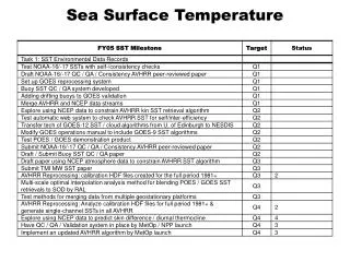
6. Observation and Background Error Variances • Statistical analysis performed on month-long sample of observations across CONUS • See paper for details; same method used by Myrick and Horel (2006) • Results of analysis show σo2:σb2 should be doubled (2:1)

7. Background Error Covariance: Example Correlation - Winchester, VA R = 40 km, Z = 100 m R = 80 km, Z = 200 m 0.3 0.4 0 0.1 0.2 0.5 0.6 0.7 0.8 0.9 1.0

8. Data Denial Methodology • Evaluation of analyses done by randomly withholding observations • Two error measures: • Root-mean-square error (RMSE) calculated at the observation gridpoints • Root-mean-square sensitivity computed across all gridpoints • Measures need observations that are randomly distributed across the grid to be effective

9. Hilbert Curve Withholding Methodology

10. Shenandoah Valley Case Study • 4°x4° area centered over Shenandoah Valley, VA • Shenandoah Valley between Blue Ridge Mtns. And Appalachian Mtns. • Washington, D.C. located in eastern part of domain KIAD Appalachian Mountains Shenandoah Valley Washington, D.C. Blue Ridge Mountains 0 100 200 300 400 500 600 700 800 900 1000

11. Case Study: Synoptic Situation 1200 UTC 22 October 2007 KIAD • Analyzing analysis generated for 0900 UTC 22 October 2007 • Strong surface inversion up to 1500 m in morning sounding

12. Case Study: Background Field • Downscaling leads southwest-northwest oriented bands • Observations provide detail along mountain slopes and in Shenandoah Valley 6 2 3 4 5 11 16 17 7 8 9 10 12 13 14 15

13. Case Study: Observations METAR 16/59/1,744 OTHER 10/75/1,961 PUBLIC 215/575/6,486 RAWS 3/11/1,301

14. LSA Analyses R = 40 km, Z = 100 m, σo2/σb2 = 1 R = 80 km, Z = 200 m, σo2/σb2 = 2 6 11 16 17 2 3 4 5 8 9 10 12 13 14 15 7

15. LSA Analysis Increments R = 40 km, Z = 100 m, σo2/σb2 = 1 R = 80 km, Z = 200 m, σo2/σb2 = 2 -3 5 -5 -4 -1 0 1 2 3 4 -2

16. Data Denial Example • Data denial methodology applied using 10 observation sets • RMSE and Sensitivity computed for each set of analysis characteristics • Right: Difference between control analysis and data withheld analysis • Blue (red) means control analysis was colder (warmer) than withheld 2 -2.5 -2 -1.5 -1 -0.5 0 0.5 1 1.5 2.5

17. Results Measure of analysis quality in data rich areas Measure of analysis quality in data voids

18. Summary • Local 2D-Var surface analysis developed for this research • Ratio of observation to background error variance and decorrelation length scales larger than previously assumed • Analysis of RMSE values using withheld observations and all observations provides a measure of analysis overfitting • For further information, see full article submitted to WAF for review

19. Extra Slides

20. Specification of Observation Error Variance and Background Error Covariance • Statistical analysis using month long sample to estimate error variances • See Myrick and Horel 2006 • Background error covariance specified in terms of spatial distance: • Estimation shows a σo2:σb2 of 2:1 and horiz. and vert. decorrelation length scales of 80 km and 200 m