Download
1 / 42
430 likes | 601 Views
Low Power Techniques in FIR Filters. Mohsen Saneei DSP Implementation Systems Course Seminar. Spring 83. Outline. Power Elements Block diagram of an FIR filter Number Representation techniques for low power Reduced 2’SC Representation Mixed Number Representation Bus coding

E N D
Low Power Techniques in FIR Filters Mohsen Saneei DSP Implementation Systems Course Seminar Spring 83
Outline • Power Elements • Block diagram of an FIR filter • Number Representation techniques for low power • Reduced 2’SC Representation • Mixed Number Representation • Bus coding • Gray Code addressing • Bus Invert Coding • Bus Bit Reordering • Parallel Processing and Pipelining
Outline (cont.) • Low power technique in FIR filters • Coefficient Scaling • Reduced Number of Multiplications in Linear Phase Filters • Coefficient Optimization • Using Differential Coefficients • Multi-rate Architectures • Coefficient and Data Swapping in Booth Multipliers • Selective Coefficient Negation • Coefficient Ordering • Adder input Bit Swapping • Coefficient Segmentation Algorithm • Data Block Processing • Transposed Direct form Implementation • Use of Multiple Multiplier (2’SC or SM)
1) Power Elements • Sources of power dissipation in CMO circuits: • Switching power • Short-circuit power • Leakage power • Switching power (Dynamic Power): Pdynamic = αT . Cswitch . V2 . fclk
2) Block diagram of an FIR filter (cont.) AU for the conventional filter Using 2’SC data and coefficient AU for the conventional filter Using SM data and coefficient
3-1) Reduced 2’SC Representation [1] X=xN-1…x2x1x0 +3=00000011 3-4=11111111 X= x’m-1xm-2….x2x1x0 + 1 1 . . . . 1 1 :correction vector ------------------------------------------------- X=xm-1xm-1 . . . xm-1xm-1xm-2….x2x1x0 -3=11111101=00000001+ 111111 -------------------
3-1) Experimental Results: • 0.25 µm CMOS • 160 taps (8 taps per hybrid section • 100 MHz clock speed • 10 bit coefficient • 2.5 V Power supply • 6 mm2 core size • Power dissipation: • 200 mW in dynamic reduced Representation mode • 295 mW in fixed word-length reduced Representation mode • Power saving: 32%
3-1) Another examples: • Booth-Encoding Multiplier: • Transposed Form Feed-Forward Equalization Filter • 2’SC: 105.6 mW • Reduced Rep: 78.8 mW • Power saving: 25%
3-2) Mixed Number Representation [2] • Multiplier:Booth encoding • Multiplicand:SM • Expected Switching Activity(ESA) • Negation of a 2’SC number: Complement all bits and then adding ‘1’ • Negation of a SM number: Complement Sign-bit • So: ESA in SM number is lower of 2’SC
3-2) The Algorithm: • Convert the multiplicand from 2’SC into the SM representation . • Apply the radix-4 Booth’s algorithm to Multiplier and generate all the PPs representation in SM notation. • Convert all the partial products from SM into RB representation • Sum up all the PPs through a RB adder tree. • Convert the final result from RB into 2’SC notation
4-1) Gray Code addressing [3] • For Gray Code , Hamming distance in sequential number is 1. • During the FIR filter computation, both the coefficient and the data are accessed sequentially. • So gray code is approach for address bus encoding.
4-3) Bus Bit Reordering [3] % Reduction in the number of adjacent signal transitions in opposite direction as a function of the bus-reordering span
6-1) Coefficient Scaling [3] • Scale coefficient of the filter • An optimal scaling factor K can be found such that the total Hamming distance between consecutive coefficient value is minimized.
6-2) Reduced Number of Multiplications in Linear Phase Filters [3] • The coefficient symmetry of linear phase FIR filters can be used to reduced by half the number of multiplication per output. N multiplication reduced to N/2 multiplication
6-3) Coefficient Optimization [3] • Given a N-tap filter with coefficient hi that satisfy the response in terms of pass-band ripple, stop-band attenuation. • Find a new set of coefficient ki.hi such that the total hamming distance between successive coefficient is minimized while still satisfying the desired filter characteristics.
Hamming distance and adjacent signal toggles after coefficient scaling and optimization
6-4) Using Differential Coefficients [6] Yn-2 = h0xn-2 + h1xn-3+ h2xn-4 + h3xn-5 Yn-1 = h0xn-1 + h1xn-2 + h2xn-3 + h3xn-4 Yn = h0xn + h1xn-1 + h2xn-2 + h3xn-3 h1xn-1 = h0xn-1 + (h1-h0)xn-1 h3xn-3 = h2xn-3 + (h3-h2)xn-3 h2xn-2 = h1xn-2 + (h2-h1)xn-2 h1xn-2 = h0xn-2 + (h1-h0)xn-2
6-5) Multi-rate Architectures [3] • Results: • A N-tap direct form architecture requires: • N multiplication and (N-1) addition per output • But, A N-tap multi-rate architecture requires: • 3N/4 multiplication and (3N+2)/4 addition per output • 30 – 50% power saving X(z)=Xe(z) + z-1Xo(z) Y(z)=Ye(z) + z-1Yo(z) H(z)=He(z) + z-1Ho(z)
6-6) Coefficient and Data Swapping in Booth Multipliers [3] • Power dissipation in a Booth multiplier depends on the number of “1’s” in the Booth encoded input. • So, coefficient and data inputs to the multiplier can be appropriately swapped so as to reduced power dissipation in the multiplier.
6-7) Selective Coefficient Negation [3] • For each coefficient hi, either hi or –hi stored in the coefficient memory. • Adder replaced with an adder/substructure. • Result: • reduces the number of 1 in the coefficient input • Reduces Hamming distance between consecutive coefficient
6-8) Coefficient Ordering [3] • Summation operation is commutative and associative • So: Yn = h0xn + h1xn-1 + h2xn-2 + h3xn-3 = h1xn-1 + h3xn-3+h0xn+ h2xn-2 • We can exchange the order of coefficient and data in memory to achieve minimum hamming distance.
Hamming distance and adjacent signal toggles after coefficient selective negation, scaling and Ordering
6-10) Coefficient Segmentation Algorithm [7] • Coefficient set = {h0,h1,h2,h3,…,hN-1} • For a given coefficient hk, the algorithm targets dividing it such that hk = sk + mk, where • sk is the largest power of 2 smaller than hk . • mk = hk-sk is a positive number. • hk . xk = sk . xk + mk . Xk shift multiply
6-11) Data Block Processing[8] Yn-1 = h0xn-1 + h1xn-2 + h2xn-3 + h3xn-4 Yn = h0xn + h1xn-1 + h2xn-2 + h3xn-3
6-12)Transposed Direct form implementation (TDF)[3, 9] • In DF: for each multiplication both input of the multiplier receive new data. • In TDF: the data input of the multiplier remains unchanged for a substantial number of multiplication operation, corresponding to the filter length • So: reduced SA in data bus and data input of multiplier Direct Form Transposed Direct Form
Use of Multiple Multiplier (2’SC or SM) 2’SC and DF SM representation and TDF
Use of Multiple Multiplier (2’SC or SM) Result of a BPF with 64-tap (2’SC) DF: Direct Form TDF: Transpose Direct Form Norm: normal Min: minimum Hamming distance
References • Zhan Yu, Meng-Lin Yu, Kamran Azadet and Alen N. Willson Jr: “the use of reduced two's complement representation in low power DSP design” , IEEE 2002 • M. Zheng and A. Albicki: ” Low power and high speed multiplication design through mixed number representation” , IEEE 1995 • M. Mehendale , S. D. Sherlekar and G. Venkatesh: “Low-Power Realization of FIR Filters on Programmable DSP’s” , IEEE Transaction on very large scale integration (VLSI) system, Vol. 6 , NO. 4, December 1998 • M. R. Stan, W. P. Burleson: “Bus-Invert Coding for Low Power I/O” , IEEE Transaction on very large scale integration (VLSI) system, Vol. 3 , NO. 1, March 1995 • A. P. Chandrakasan , R. W. Brodersen: “ Minimizing Power Consumption in Digital CMOS Circuits” , Proceeding of the IEEE, Vol. 83, NO. 4 , April 1995
References (cont.) • N. Sankarayya, Kaushik Roy, and Debashis Bhattacharya: “Algorithms for Low Power and High Speed FIR Filter Realization Using Differential Coefficients” , IEEE TRANSACTIONS ON CIRCUITS AND SYSTEMS—II: ANALOG AND DIGITAL SIGNAL PROCESSING, VOL. 44, NO. 6, JUNE 1997 • A. T. Erdogan and T. Arslan: “A Coefficient Segmentation Algorithm for Low Power Implementation of FIR filters” IEEE 1999 • A.T. Erdogan and T. Arslan: “LOW POWER BLOCK BASED FIR FILTERING CORES”, ISCAS-2003 • A.T. Erdogan and T. Arslan: “high throughput FIR filter design for low power SoC applications”, IEEE 2000 • A.T. Erdogan and T. Arslan: “low power implementation of high throughput FIR filter”, IEEE 2002