Download

1 / 22
220 likes | 320 Views
Turbulence and Mixing in Shelf Seas John Simpson, Tom Rippeth, Neil Fisher,Mattias Green Eirwen Williams, Phil Wiles, Matthew Palmer Funded by the NERC, EU (OAERRE, MABENE, C2C) and Dstl With technical support from Ray Wilton, Ben Powell & the officers and crew of the Prince Madog .

E N D
Turbulence and Mixing in Shelf Seas John Simpson, Tom Rippeth, Neil Fisher,Mattias Green Eirwen Williams, Phil Wiles, Matthew Palmer Funded by the NERC, EU (OAERRE, MABENE, C2C) and Dstl With technical support from Ray Wilton, Ben Powell & the officers and crew of the Prince Madog . School of Ocean Sciences, University of Wales Bangor, Menai Bridge, LL59 5EY, UK Ysgol Gwyddorau Eigion, Prifysgol Cymru Bangor, Porthaethwy Visit our web site at: www.sos.bangor.ac.uk/research/tmiss/index.html
Menu • Motivation • Measurement capabilities • Mapping ε in shelf regimes with FLY • ADCP variance method for Production • Mixing in the pycnocline of the shelf seas
Motivation ? Key environmental control of: Fluxes of nutrients/ particles etc. (Mixing) Particle aggregation/disaggregation Predator-prey encounter rates Tests of Turbulence Closure schemes for models Turbulent processes in shelf seas
Which Properties ?DiffusionTKE productionBuoyancyDissipation ADCP Variance method
FLY Dissipation Profiler
S1 M1
Mixed station M1 observed ε Time(days) ε Model MY2.2 (with diffusion) Model MY2.0 (no diffusion)
Stratified station S1 T°C ε (Wm-3)
ε observed ε Model MY2.2
Model – Observation Inter-comparison Model • BIG discrepancy between the predicted (using MY2.2 closure scheme) and observed levels of e(Simpson et al., 1996). • ie. The model fails to reproduce the critical dissipation and thus mixing within the thermocline. S1 Obs. Bottom Boundary Layer Log10 [e0 (Wm-3)] Missing physical processes within the model?
The phase of TKE production ? The velocity shear in a boundary layer forced by an oscillating pressure gradient X=A cos ωt is given by (Lamb p.622): The corresponding TKE production will be: So that the production (and hence ε ) will exhibit an M4 phase lag of : which increase with height above bed at a rate
AMPLITUDE PHASE Mixed Nz=0.4m2s-1 Mixed Nz=0.13m2s-1 Stratified Nz=0.025m2s-1 Phase lag (hours)
LB2 Temperature Salinity
Log W/m3 Cycle of epsilon with density JPO 31,2458-2471 (2001)
GOT Model k-epsilon +Canuto Hans Burchard Karsten Bolding
P/ε B/ε
z v4 w4 b4 4 3 y ADCP Variance Method