Download

1 / 18
180 likes | 290 Views
Community Ecology BDC331. Mark J Gibbons, Room 4.102, BCB Department, UWC Tel: 021 959 2475. Email: mgibbons@uwc.ac.za. Content acknowledgements – Dr Vanessa Couldridge, UWC. For Example………. What patterns can see when you look at the above data?. Correlation and linear regression.

E N D
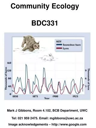
Community Ecology BDC331 Mark J Gibbons, Room 4.102, BCB Department, UWC Tel: 021 959 2475. Email: mgibbons@uwc.ac.za Content acknowledgements – Dr Vanessa Couldridge, UWC
For Example……….. What patterns can see when you look at the above data? Correlation and linear regression When trying to explain some of the patterns you have observed in your species and community data, it sometimes helps to have a look at relationships between variables – both physical and biological Is it possible to quantify your observations?
Correlation and linear regression: not the same, but are related Correlation: quantifies how X and Y vary together Linear regression: line that best predicts Y from X Use correlation when both X and Y are measured Use linear regression when one of the variables is controlled
3 characteristics of a relationship Direction Positive(+) Negative ( - ) Degree of association Between – 1 and +1 Absolute values signify strength Form Linear Non - linear Direction Positive Negative C1 vs C2 C1 vs C2 120.0 20.0 80.0 13.3 C2 C2 40.0 6.7 0.0 0.0 0.0 4.0 8.0 12.0 0.0 83.3 166.7 250.0 C1 C1 Large values of X = large values of Y, Large values of X = small values of Y Small values of X = small values of Y. Small values of X = large values of Y e.g., height and weight e.g., speed and accuracy
Degree of association Strong Weak (tight cloud) (diffuse cloud) C1 vs C2 C1 vs C2 120.0 20.0 80.0 13.3 C2 C2 40.0 6.7 0.0 0.0 0.0 4.0 8.0 12.0 0.0 4.0 8.0 12.0 C1 C1 Form Linear Non - linear
Dataset Obs X Y A 1 1 B 1 3 C 3 2 D 4 5 E 6 4 F 7 5 Pearson’s r A value ranging from -1.00 to 1.00 indicating the strength and direction of the linear relationship Absolute value indicates strength +/ - indicates direction : a statistical technique that measures and Correlation describes the degree of linear relationship between two variables Scatterplot Y X
= r √ Remember……………. (X – X)(Y – Y) Sum of Squares (Sample) Σ 2 Mean Sum of Squares (sample) (Variance) (Y – Y) N mean 2 (X – X) Square units? √ (Variance) Standard Deviation 16 s = 1.5 2.25 How to Calculate Pearson’s r
= r √ 2 2 (Y – Y) (X – X) covariation of X, Y = r total variation of X, Y (X – X)(Y – Y) Means this in words……… The equation for r NUMERATOR: For each set of X and Y values - you are looking at the deviation of X from its mean, and the deviation of Y from its mean – to get a feel for their joint deviation – or covariation. This is summed across all sets of X-Y values to provide an overall index of co-variation. DENOMINATOR: This is simply total variation of X and Y (see previous slide)
= r √ (X – X)(Y – Y) 2 (Y – Y) 2 (X – X) For Example…………. = 834 / √(696.8 x 10¹⁰) = 834 / √703768 = 834 / 383.9 = 0.994
Outliers Child 19 is lowering r Child 18 is increasing r Some issues with r Outliers have strong effects Restriction of range can suppress or augment r Correlation is not causation No linear correlation does not mean no association
The restricted range problem The relationship you see between X and Y may depend on the range of X For example, the size of a child’s vocabulary has a strong positive association with the child’s age But if all of the children in your data set are in the same grade in school, you may not see much association Common causes, confounds Two variables might be associated because they share a common cause. There is a positive correlation between ice cream sales and the number of drowning incidents. . Also, in many cases, there is the question of reverse causality
50 45 40 35 30 Proficiency 25 20 15 10 5 0 1 2 3 4 5 6 Practice time Non - linearity Some variables are not linearly related, though a relationship obviously exists
The correlation coefficient, r, is a statistic It summarises the co-variation or correlation between the two variables and varies (excluding negatives) from 0 to 1 Its significance can be determined by checking it against the appropriate critical value [for a set level of probability, degree of freedom and alpha (1 or 2 tailed)] in a table of r values. When you check the table – ignore the sign of your value If your value is greater than the critical value, then it is considered significant. Before checking it, however, you need to set up a null hypothesis (H0) What would such an hypothesis be?
The amount of covariation compared to the amount of total variation “The percent of total variance that is shared variance” E.g. “If r = .80, then X explains 64% of the variability in Y” (and vice versa) If r is the correlation coefficient, what is r2? MSExcel can generate r2 values…………….
r = 0.93 r = 0.911 BUT…….. r = 0.302 A CAUTIONARY NOTE
THE END Content acknowledgements – Dr Vanessa Couldridge, UWC Image acknowledgements – http://www.google.com