Download
1 / 45
450 likes | 688 Views
EEEM048- Internet of Things Lecture 6- Intelligent Data Processing. Dr Payam Barnaghi, Dr Chuan H Foh Centre for Communication Systems Research Electronic Engineering Department University of Surrey Autumn Semester 2013/2014. Wireless Sensor (and Actuator) Networks.

E N D
EEEM048- Internet of Things Lecture 6- Intelligent Data Processing Dr Payam Barnaghi, Dr Chuan H Foh Centre for Communication Systems Research Electronic Engineering Department University of Surrey Autumn Semester 2013/2014
Wireless Sensor (and Actuator) Networks Inference/Processing of IoT data Services? End-user Operating Systems? Protocols? Core network e.g. Internet Protocols? Gateway Data Aggregation/ Fusion In-node Data Processing Sink node Gateway Computer services • The networks typically run Low Power Devices • Consist of one or more sensors, could be different type of sensors (or actuators)
Key characteristics of IoT devices • Often inexpensive sensors (actuators) equipped with a radio transceiver for various applications, typically low data rate ~ 10-250 kbps. • Deployed in large numbers • The sensors should coordinate to perform the desired task. • The acquired information (periodic or event-based) is reported back to the information processing centre (or some cases in-network processing is required) • Solutions are often application-dependent. 3
Beyond conventional sensors • Human as a sensor (citizen sensors) • e.g. tweeting real world data and/or events • Software sensors • e.g. Software agents/services generating/representing data Road block, A3 Road block, A3 Suggest a different route
The benefits of data processing in IoT Turn 12 terabytes of Tweets created each day into sentiment analysis related to different events/occurrences or relate them to products and services. Convert (billions of) smart meter readings to better predict and balance power consumption. Analyze thousands of traffic, pollution, weather, congestion, public transport and event sensory data to provide better traffic and smart city management. Monitor patients, elderly care and much more… Requires: real-time, reliable, efficient (for low power and resource limited nodes), and scalable solutions. Partially adapted from: What is Bog Data?, IBM
IoT Data Access Publish/Subscribe (long-term/short-term) Ad-hoc query The typical types of data request for sensory data: Query based on ID (resource/service) – for known resources Location Type Time – requests for freshness data or historical data; One of the above + a range [+ Unit of Measurement] Type/Location/Time + A combination of Quality of Information attributes An entity of interest (a feature of an entity on interest) Complex Data Types (e.g. pollution data could be a combination of different types)
Sensor Data The sensory data represents physical world observation and measurement and requires time and location and other descriptive attributes to make the data more meaningful. For example, a temperature value of 15 degree will be more meaningful when it is described with spatial (e.g. Guildford city centre) and temporal (e.g. 8:15AM GMT, 21-03-2013), and unit (e.g. Celsius) attributes. The sensory data can also include other detailed meta-data that describe quality or device related attributes (e.g. Precision, Accuracy).
Sensor Data 15, C, 08:15, 51.243057, -0.589444
“Raw data is both an oxymoron and bad data” Geoff Bowker, 2005 Source: Kate Crawford, "Algorithmic Illusions: Hidden Biases of Big Data", Strata 2013.
Data Processing and Interpretation Intelligent Processing and Interpretation of data (this week) Meta-data enhancement, annotation and semantically described IoT data(next week)
IoT Data Challenges Interoperability: various data in different formats, from different sources (and different qualities) Discovery: finding appropriate device and data sources Access: Availability and (open) access to resources and data Search: querying for data Integration: dealing with heterogeneous device, networks and data Interpretation: translating data to knowledge usable by people and applications Scalability: dealing with large number of devices and myriad of data and computational complexity of interpreting the data.
IoT Data in the Cloud Image courtesy: http://images.mathrubhumi.com http://www.anacostiaws.org/userfiles/image/Blog-Photos/river2.jpg
Comparing IoT data streams with conventionalmultimedia streams Source: P. Barnaghi, W. Wang, L. Dong, C. Wang, "A Linked-data Model for Semantic Sensor Streams", in the Proc. of IEEE International Conference on Internet of Things (iThings 2013), August 2013.
IoT Data Processing WSN WSN WSN WSN WSN Network-enabled Devices Data collections and processing within the networks Network-enabled Devices Network services/storage and processing units Data/service access at application level Data Discovery Service/Resource Discovery
In-network processing • Mobile Ad-hoc Networks can be seen as a set of nodes that deliver bits from one end to the other; • WSNs, on the other end, are expected to provide information, not necessarily original bits • Gives additional options • e.g., manipulate or process the data in the network • Main example: aggregation • Applying aggregation functions to a obtain an average value of measurement data • Typical functions: minimum, maximum, average, sum, … • Not amenable functions: median Source: Protocols and Architectures for Wireless Sensor Networks, Protocols and Architectures for Wireless Sensor Networks Holger Karl, Andreas Willig, chapter 3, Wiley, 2005 .
In-network processing Depending on application, more sophisticated processing of data can take place within the network Example edge detection: locally exchange raw data with neighboring nodes, compute edges, only communicate edge description to far away data sinks Example tracking/angle detection of signal source: Conceive of sensor nodes as a distributed microphone array, use it to compute the angle of a single source, only communicate this angle, not all the raw data Exploit temporaland spatial correlation Observed signals might vary only slowly in time; so no need to transmit all data at full rate all the time Signals of neighboring nodes are often quite similar; only try to transmit differences (details a bit complicated, see later) Source: Protocols and Architectures for Wireless Sensor Networks, Protocols and Architectures for Wireless Sensor Networks Holger Karl, Andreas Willig, chapter 3, Wiley, 2005 .
Data-centric networking In typical networks (including ad-hoc networks), network transactions are addressed to the identitiesof specific nodes A “node-centric” or “address-centric” networking paradigm In a redundantly deployed sensor networks, specific source of an event, alarm, etc. might not be important Redundancy: e.g., several nodes can observe the same area Thus: focus networking transactions on the data directly instead of their senders and transmitters ! data-centric networking Specially this idea is reinforced by the fact that we might have multiple sources to provide information and observations form the same or similar areas. Principal design change Source: Protocols and Architectures for Wireless Sensor Networks, Protocols and Architectures for Wireless Sensor Networks Holger Karl, Andreas Willig, chapter 3, Wiley, 2005 .
Data-centric networking in WSN Data in WSN is often transient (or at least time dependent) Spatial feature of data is important Quality of information can vary (depending on sources and also the environment changes) In large-scale deployments, there could be large number of small information (in contrast to conventional data-centric networks that mainly focus on large multimedia content) Data discovery (or resource discovery) is a challenge Data annotation and description frameworks e.g. Semantic sensor Networks- to annotate sensor resources and observation and measurement data (more on this topic next week).
Data Aggregation • Computing a smaller representation of a number of data items (or messages) that is extracted from all the individual data items. • For example computing min/max or mean of sensor data. • More advance aggregation solutions could use approximation techniques to transform high-dimensionality data to lower-dimensionality abstractions/representations. • The aggregated data can be smaller in size, represent patterns/abstractions; so in multi-hop networks, nodes can receive data form other node and aggregate them before forwarding them to a sink or gateway. • Or the aggregation can happen on a sink/gateway node.
Aggregation example 1 1 1 1 3 1 1 1 6 1 1 1 • Reduce number of transmitted bits/packets by applying an aggregation function in the network Source: Holger Karl, Andreas Willig, Protocols and Architectures for Wireless Sensor Networks, Protocols and Architectures for Wireless Sensor Networks, chapter 3, Wiley, 2005 .
Efficacy of an aggregation mechanism • Accuracy: difference between the resulting value or representation and the original data • Some solutions can be lossless or lossly depending on the applied techniques. • Completeness: the percentage of all the data items that are included in the computation of the aggregated data. • Latency: delay time to compute and report the aggregated data • Computation foot-print; complexity; • Overhead: the main advantage of the aggregation is reducing the size of the data representation; • Aggregation functions can trade-off between accuracy, latency and overhead; • Aggregation should happen close to the source.
Publish/Subscribe Publisher 1 Publisher 2 Subscriber 1 Subscriber 2 Subscriber 3 Software bus • Achieved by publish/subscribe paradigm • Idea: Entities can publish data under certain names • Entities can subscribe to updates of such named data • Conceptually: Implemented by a software bus • Software bus stores subscriptions, published data; names used as filters; subscribers notified when values of named data changes • Variations • Topic-based P/S – inflexible • Content-based P/S – use general predicates over named data Source: Holger Karl, Andreas Willig, Protocols and Architectures for Wireless Sensor Networks, Protocols and Architectures for Wireless Sensor Networks, chapter 12, Wiley, 2005 .
MQTT Pub/Sub Protocol • MQ Telemetry Transport (MQTT) is a lightweight broker-based publish/subscribe messaging protocol. • MQTT is designed to be open, simple, lightweight and easy to implement. • These characteristics make MQTT ideal for use in constrained environments, for example in IoT. • Where the network is expensive, has low bandwidth or is unreliable • When run on an embedded device with limited processor or memory resources; • A small transport overhead (the fixed-length header is just 2 bytes), and protocol exchanges minimised to reduce network traffic • MQTT was developed by Andy Stanford-Clark of IBM, and Arlen Nipper of Cirrus Link Solutions. Source: MQTT V3.1 Protocol Specification, IBM, http://public.dhe.ibm.com/software/dw/webservices/ws-mqtt/mqtt-v3r1.html
MQTT • It supports publish/subscribe message pattern to provide one-to-many message distribution and decoupling of applications • A messaging transport that is agnostic to the content of the payload • The use of TCP/IP to provide basic network connectivity • Three qualities of service for message delivery: • "At most once", where messages are delivered according to the best efforts of the underlying TCP/IP network. Message loss or duplication can occur. • This level could be used, for example, with ambient sensor data where it does not matter if an individual reading is lost as the next one will be published soon after. • "At least once", where messages are assured to arrive but duplicates may occur. • "Exactly once", where message are assured to arrive exactly once. This level could be used, for example, with billing systems where duplicate or lost messages could lead to incorrect charges being applied. Source: MQTT V3.1 Protocol Specification, IBM, http://public.dhe.ibm.com/software/dw/webservices/ws-mqtt/mqtt-v3r1.html
MQTT Message Format • The message header for each MQTT command message contains a fixed header. • Some messages also require a variable header and a payload. • The format for each part of the message header: • DUP: Duplicate delivery • QoS: Quality of Service • RETAIN: RETAIN flag • This flag is only used on PUBLISH messages. When a client sends a PUBLISH to a server, if the Retain flag is set (1), the server should hold on to the message after it has been delivered to the current subscribers. • This allows new subscribers to instantly receive data with the retained, or Last Known Good, value. Source: MQTT V3.1 Protocol Specification, IBM, http://public.dhe.ibm.com/software/dw/webservices/ws-mqtt/mqtt-v3r1.html
Sensor Data as time-series data • The sensor data (or IoT data in general) can be seen as time-series data. • A sensor stream refers to a source that provide sensor data over time. • The data can be sampled/collected at a rate (can be also variable) and is sent as a series of values. • Over time, there will be a large number of data items collected. • Using time-series processing techniques can help to reduce the size of the data that is communicated; • Let’s remember, communication can consume more energy than communication;
Sensor Data as time-series data • Different representation method that introduced for time-series data can be applied. • The goal is to reduce the dimensionality (and size) of the data, to find patterns, detect anomalies, to query similar data; • Dimensionality reduction techniques transform a data series with n items to a representation with w items where w < n. • This functions are often lossy in comparison with solutions like normal compression that preserve all the data. • One of these techniquesis called Symbolic Aggregation Approximation (SAX). • SAX was originally proposed for symbolic representation of time-series data; it can be also used for symbolic representation of time-series sensor measurements. • The computational foot-print of SAX is low; so it can be also used as a an in-network processing technique.
In-network processing UsingSymbolic Aggregate Approximation (SAX) fggfffhfffffgjhghfff jfhiggfffhfffffgjhgi fggfffhfffffgjhghfff SAX Pattern (blue) with word length of 20 and a vocabulary of 10 symbols over the original sensor time-series data (green) Source: P. Barnaghi, F. Ganz, C. Henson, A. Sheth, "Computing Perception from Sensor Data", in Proc. of the IEEE Sensors 2012, Oct. 2012.
Symbolic Aggregate Approximation (SAX) • SAX transforms time-series data into symbolic string representations. • Symbolic Aggregate approXimation was proposed by Jessica Lin et al at the University of California –Riverside; • http://www.cs.ucr.edu/~eamonn/SAX.htm . • It extends Piecewise Aggregate Approximation (PAA) symbolic representation approach. • SAX algorithm is interesting for in-network processing in WSN because of its simplicity and low computational complexity. • SAX provides reasonable sensitivity and selectivity in representing the data. • The use of a symbolic representation makes it possible to use several other algorithms and techniques to process/utilise SAX representations such as hashing, pattern matching, suffix trees etc.
Processing Steps in SAX • SAX transforms a time-series X of length n into the string of arbitrary length, where typically, using an alphabet A of size a > 2. • The SAX algorithm has two main steps: • Transforming the original time-series into a PAA representation • Converting the PAA intermediate representation into a string during. • The string representations can be used for pattern matching, distance measurements, outlier detection, etc.
Piecewise Aggregate Approximation • In PAA, to reduce the time series from ndimensions to wdimensions, the data is divided into w equal sized “frames.” • The mean value of the data falling within a frame is calculated and a vector of these values becomes the data-reduced representation. • Before applying PAA, each time series to have a needs to be normalised to achieve a mean of zero and a standard deviation of one. • The reason is to avoid comparing time series with different offsets and amplitudes; Source: Jessica Lin, Eamonn Keogh, Stefano Lonardi, and Bill Chiu. 2003. A symbolic representation of time series, with implications for streaming algorithms. In Proceedings of the 8th ACM SIGMOD workshop on Research issues in data mining and knowledge discovery (DMKD '03). ACM, New York, NY, USA, 2-11.
SAX- normalisation before PAA Timeseries (c): 2, 3, 4.5, 7.6, 4, 2, 2, 2, 3, 1 Mean (μ):μ= (2+3+4.5+7.6+4+2+2+2+3+1)/10= 3.11 Standard deviation (σ): (2-3.11)2 = 1.2321 (3-3.11)2 = 0.0121 (4.5-3.11)2 = 1.9321 (7.6-3.11)2 = 20.1601 (4-3.11)2 = 0.7921 (2-3.11)2 = 1.2321 (2-3.11)2 = 1.2321 (2-3.11)2 = 1.2321 (3-3.11)2 = 0.0121 (1-3.11)2 = 4.4521 1.2321+0.0121+ 1.9321+ 20.1601+ 0.7921+ 1.2321+ 1.2321+ 1.2321+ 1.2321+ 0.0121+4.4521 = 33.5211 σ = √ (33.5211/10) = 1.83087683911
Normalisation Timeseries (c): 2, 3, 4.5, 7.6, 4, 2, 2, 2, 3, 1 Normalised: zi = (ci – μ)/ σ σ = 1.83087683911 μ = 3.11 z1 = (2- 3.11)/1.83087683911 = -0.606 z2 = (3-3.11)/ 1.83087683911= -0.600 z3 = (4.5-3.11)/ 1.83087683911= 2.452 z4 = (7.6-3.11)/ 1.83087683911= -0.600 z5 = (4-3.11)/ 1.83087683911= 0.486 z6 = (2-3.11)/ 1.83087683911= -0.606 z7 = (2-3.11)/ 1.83087683911= -0.606 z8 = (2-3.11)/ 1.83087683911= -0.606 z9 = (3-3.11)/ 1.83087683911= -0.600 z10 = (1-3.11)/ 1.83087683911= -1.152 Normalised Timeseries (z): -0.606, -0.600, 2.452, -0.600, 0.486, -0.606, -0.606, -0.606 , -0.600, -1.152
PAA calculation Timeseries (c): 2, 3, 4.5, 7.6, 4, 2, 2, 2, 3, 1 Normalised Timeseries (z): -0.606, -0.600, 2.452, -0.600, 0.486, -0.606, -0.606, -0.606 , -0.600, -1.152 PAA (w=5): -0.603, 0.926, -0.06, -0.606, 0.273
PAA to SAX Conversion • Conversion of the PAA representation of a time-series into SAX is based on producing symbols that correspond to the time-series features with equal probability. • The SAX developers have shown that time-series which are normalised (zero mean and standard deviation of 1) follow a Normal distribution (Gaussian distribution). • The SAX method introduces breakpoints that divides the PAA representation to equal sections and assigns an alphabet for each section. • For defining breakpoints, Normal inverse cumulative distribution function
Breakpoints in SAX • “Breakpoints: breakpoints are a sorted list of numbers B = β1,…, βa-1 such that the area under a N(0,1) Gaussian curve from βi to βi+1 = 1/a”. Source: Jessica Lin, Eamonn Keogh, Stefano Lonardi, and Bill Chiu. 2003. A symbolic representation of time series, with implications for streaming algorithms. In Proceedings of the 8th ACM SIGMOD workshop on Research issues in data mining and knowledge discovery (DMKD '03). ACM, New York, NY, USA, 2-11.
Alphabet representation in SAX • Let’s assume that we will have 4 symbols alphabet: a,b,c,d • As shown in the table in the previous slide, the cut lines for this alphabet (also shown as the thin red lines on the plot below) will be { -0.67, 0, 0.67 } Source: JMOTIF Time series mining, http://code.google.com/p/jmotif/wiki/SAX
SAX Represetantion Timeseries (c): 2, 3, 4.5, 7.6, 4, 2, 2, 2, 3, 1 Normalised Timeseries (z): -0.606, -0.600, 2.452, -0.600, 0.486, -0.606, -0.606, -0.606 , -0.600, -1.152 PAA (w=5): -0.603, 0.926, -0.06, -0.606, 0.273 Cut off ranges: {-0.67, 0, 0.67} Alphabet: a ,b ,c, d SAX representation: bdbbc
Features of the SAX technique • SAX divides a time series data into equal segments and then creates a string representation for each segment. • The SAX patterns create the lower-level abstractions that are used to create the higher-level interpretation of the underlying data. • The string representation of the SAX mechanism enables to compare the patterns using a specific type of string similarity function.
A sample data processing framework On going meeting Window has been left open High-level information/knowledge Spatial data (extracted from descriptions) Temporal data (extracted from descriptions) High-level abstractions Domain knowledge Office room BA0121 Day-time Intelligent Processing/Reasoning Intelligent Processing … Night-time …. …. Observations Thematic data (low level abstractions) Attendance Phone Hot Temperature Cold Temperature Bright SAX Patterns fggfffhfffffgjhghfff dddfffffffffffddd cccddddccccdddccc dddcdcdcdcddasddd aaaacccaaaaaaaacccc Raw sensor data stream Raw sensor data stream Raw sensor data stream Raw sensor data (or Annotated data) PIR Sensor Light Sensor Temperature Sensor
Interpretation of data A primary goal of interconnecting devices and collecting/processing data from them is to create situation awareness and enable applications, machines, and human users to better understand their surrounding environments. The understanding of a situation, or context, potentially enables services and applications to make intelligent decisions and to respond to the dynamics of their environments. Next week, more on annotation and interpretation of data,.
Quiz • Consider this sensor measurements from a stream: • C = 2,3,5,0,1,3,2,0 • Calculate the normalised time series. • Calculate PAA (w=3) • Calculate SAX (alphabet size =3)
Acknowledgements • Some parts of the content are adapted from: • Holger Karl, Andreas Willig, Protocols and Architectures for Wireless Sensor Networks, Protocols and Architectures for Wireless Sensor Networks, chapters 3 and 12, Wiley, 2005 . • Jessica Lin, Eamonn Keogh, Stefano Lonardi, and Bill Chiu. 2003. A symbolic representation of time series, with implications for streaming algorithms. In Proceedings of the 8th ACM SIGMOD workshop on Research issues in data mining and knowledge discovery (DMKD '03). ACM, New York, NY, USA, 2-11. • JMOTIF Time series mining, http://code.google.com/p/jmotif/wiki/SAX