Download
1 / 42
420 likes | 790 Views
Course outline I. Introduction Game theory Price setting monopoly oligopoly Quantity setting monopoly oligopoly Process innovation. Homogeneous goods. Monopoly (quantity setting). Inverse demand function Revenues, costs, profits Profit maximizing quantity Basic model

E N D
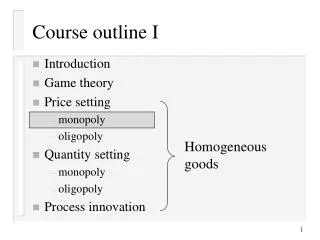
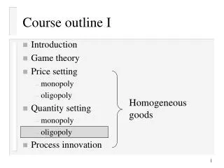
Course outline I • Introduction • Game theory • Price setting • monopoly • oligopoly • Quantity setting • monopoly • oligopoly • Process innovation Homogeneous goods
Monopoly (quantity setting) • Inverse demand function • Revenues, costs, profits • Profit maximizing quantity • Basic model • Price discrimination • Several factories • Double marginalization • Welfare analysis • Executive summary
Inverse demand function p demand function inverse demand function X
Revenue, costs and profit • Revenue: • Costs: • Profit:
Marginal revenue with respect to quantity • goes up by p (the price of the last unit), • but goes down by dp/dX X (the quantity increase diminishes the price and this price decrease is applied to all units) When a firm increases the quantity by one unit, revenue Amoroso-Robinson relation:
Marginal revenue = price? 1. i.e. horizontal demand curve, perfect competition 2. X=0 sale of first unit first degree price discrimination
Linear demand curve in a monopoly • Demand: • Revenue: • Marginal revenue:
Exercise (Depicting the linear demand curve ) • Slope of demand curve: .... • Slope of marginal revenue curve: .... • The ............................ has the same vertical intercept, ..., as the demand curve. • Economically, • the vertical intercept is ................., • the horizontal intercept is ................. .
Depicting demand and marginal revenue a 1 b 2b 1 a/(2b) a/b
First order condition • Notation:
First order condition, alternative formulations (price-cost margin)
Depicting the Cournot monopoly Cournot point
Exercise (Quantity) Consider a monopolist facing the inverse demand function p(X)=24-X. Assume that the average and marginal costs are given by AC=2. Find the profit-maximizing quantity!
Profit in a monopoly Marginal point of view: Average point of view:
Exercise (monopoly) Consider a monopoly facing the inverse demand function p(X)=40-X2. Assume that the cost function is given by C(X)=13X+19. Find the profit-maximizing price and calculate the profit.
Price discrimination • First degree price discrimination: • Second degree price discrimination: • Third degree price discrimination: Every consumer pays a different price which is equal to his or her willingness to pay. Prices differ according to the quantity demanded and sold (quantity rebate). Consumer groups (students, children, ...) are treated differently.
Monopolistic price discrimination (two markets) p p1 p2 x1 x2 total output
Inverse elasticities rule for third degree price discrimination Supplying a good X to two markets results in the inverse demand functions p1(x1) and p2(x2). Profit function: First order conditions: = Equating the marginal revenues (using the Amoroso-Robinson relation) leads to:
Exercise (two markets or one) A monopoly sells in two markets: p1(x1)=100-x1 and p2(x2)=80-x2. a) Calculate the profit-maximizing quantities and the profit at these quantities, if the cost function is given by C(X)=X2. b) Calculate the profit-maximizing quantities and the profit at these quantities, if the cost function is given by C(X)=10X. c) What happens if price discrimination between the two markets is not possible anymore? Consider C(X)=10X. Hint: Differentiate between quantities below and above 20.
Solution III (one market) 100 90 80 50 10 20 50 80 100
One market, two factories • Profit function: • First order conditions: =
One market, two factories II factory 2 factory 1 total output
Double marginalization - idea • Retailer, not producer sells to consumers. • Assumptions: • Zero costs for retailing. • Producer decides on a quantity and charges a price ppro to the retailer. • ppro is the retailer‘s marginal cost. • The retailer‘s MR=MC condition defines the producer‘s demand function.
Double marginalization - linear case • p(x)=a-bX • MCpro=ACpro=c • Second stage: First order condition for the retailer: • First stage: First order condition for the producer:
Double marginalization - depicting the solution • Producer decides on quantity and announces ppro* to retailer. • Retailer decides on quantity (fore-seen by producer). retailer producer
Double marginalization - exercise p(X)=110-X c=10 a) Calculate the price the consumers have to pay! b) What price would they pay if the producer sold directly to the consumers?
Welfare Analysis • Evaluation of economic policy measures • Welfare = consumer surplus (CS) + producer surplus (PS) + taxes - subsidies • CS = willingness to pay - price • PS = revenue - variable costs = profit + fixed costs
CS, PS - graphically supply (=MC) Welfare is maximized at the equilibrium. demand
The deadweight loss of a monopoly Without price discrimination a monopoly realizes a deadweight loss. Perfect competition
Exercise (deadweight loss) • Consider a monopoly where the demand is given by p(X)=-2X+12. Suppose that the marginal costs are given by MC=2X. • Calculate the deadweight loss • without price discrimination, • with perfect price discrimination.
Exercise (price cap in a monopoly) How does a price cap influence the demand and the marginal revenue curves?
Price cap and welfare additional welfare
Taxes on profits and welfare • Quantity / price unchanged • CS is constant • PS decrease; in the same extent net public revenues increase • deadweight loss is zero
Additional deadweight loss due to quantity tax consumer’s surplus: A+B+CA producer’s surplus: T+E+F E+B net public revenue: 0 T additional deadweight loss A C B E F T
Exercise (quantity taxes) A monopolist is facing a demand curve given by p(X)=a-X. The monopoly’s unit production cost is given by c>0. Now, suppose that the government imposes a specific tax of t dollars per unit sold. a) Show that this tax would raise the price paid by consumers by less than t.b) Would your answer change if the market inverse demand curve is given by p(X)=-ln(X)+5. c) If the demand curve is given by p(X)=X-1/2, what is the influence on price? Industrial Organization ; Oz Shy
Lerner index of monopoly power • First order condition: • Lerner index:
Monopoly profits and monopoly power Cournot point
Executive summary • A profit-maximizing monopolist always sets the quantity in the elastic region of the demand curve. • Monopolistic power: price will be set above the marginal cost by a profit maximizer. • If the demand curve is tangent to the average cost curve, the profit-maximizing price is set above marginal cost and equal to average cost. monopolistic power and zero profits • Monopolistic quantities without price discrimination (!) lead to a welfare loss. • A quantity tax leads to a welfare loss, a tax on profits does not.