Integration over the Volume

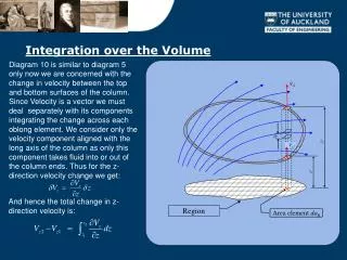
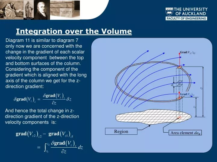
1. Integration over the Volume Diagram 11 is similar to diagram 7 only now we are concerned with the change in the gradient of each scalar velocity component between the top and bottom surfaces of the column. Considering the component of the gradient which is aligned with the long axis of the column we get for the z-direction gradient: Grad(Vz2)z2 z z2 Grad(Vz1)z1 z1 And hence the total change in z-direction gradient of the z-direction velocity components is: Region Area element daR

2. By combining this inner integration w.r.t z with an outer integration over the region we can integrate over the entire volume of the body. This leads to the result Where Fz(Visc) is the net Force in the z-direction due to the z-direction components of the z-direction velocity gradients.. Similarly for the components in the x and y directions and Now since the total net outflow Fz(visc)(total) will be given by Fz(visc)x + Fz(visc)y + Fz(visc)z it follows that:

3. Viscous Force by Volume Integration Recognising the expression: as the definition of the divergence of a field we have The div(grad) operation acting on a scalar field is called the Laplacian of the field and its symbol is 2 (pronounced Del squared) hence:

4. This can also be written as a vector in the form: This additional Diagram is of the top of the z-direction column and shows the three gradients associated with each of the three sets of scalar velocity components. Similar sets exist for each of the two horizontal columns (i.e. Those orientated in the x and y directions. Grad(Vz)z Grad(Vy)z Area = δaR Grad(Vx)z