Download
1 / 56
560 likes | 562 Views
Obtaining secondary structure from sequence. Chapter 11. Creating a Predictor The Task: what, why, how? Finding some Examples Finding some Features Making the Rules Assessing prediction accuracy Test and training datasets Accuracy measures.

E N D
Chapter 11 • Creating a Predictor • The Task: what, why, how? • Finding some Examples • Finding some Features • Making the Rules • Assessing prediction accuracy • Test and training datasets • Accuracy measures
The Task Given the sequence (primary structure) of a protein, predict its secondary structure.
Predict what? • There are many types of secondary structure. • Which do we want to predict? • Alpha helix • Beta strand • Beta turn • Random coil • Pi-helices • 310-helices • Type I turns • …
Why do it? • Is secondary structure prediction useful? • Short answer: yes • Long answer: • The original hope was to “bootstrap” from secondary to tertiary prediction; this goal remains elusive… • Secondary structure can give clues to function since many enzymes, DNA binding proteins, membrane proteins have characteristic secondary structures.
Example of importance of 2dary structure prediction • A) Signal transduction: receptor tyrosine kinase membrane-spanning alpha helix • B)G-protein-coupled receptors are important drug targets.
How can we do it? • How would you predict the secondary structure state of each residue (amino acid) in a protein? • Besides the sequence itself, what else would you want to use? • What kind of computer algorithms would help? • ???
First, get some examples to study… We need some examples of proteins with known secondary structure to try and formulate a prediction approach…
This what we want lots of… • Three examples of primary sequence labeled underneath with the secondary structure of the residue’s environment. • H=Alpha Helix, E=Beta strand, C=Coil/other
Start with some proteins of known structure • Get some good X-ray or NMR models of proteins. • Since we know their tertiary structures, certainly we can assign each residue in each protein a secondary state. • Or can we?
Is even that trivial? • Is it even trivial to label the secondary state of each residue if we know the tertiary structure? • Where does a helix begin/end? • Is that a beta sheet or not? • … • If the residue-state assignments are subjective, we’re doomed!
DSSP to the rescue! • In 1983 Kabsch and Sander introduced DSSP (Dictionary of Protein Secondary Structure) …not a typo.. • It automated the assignment of secondary structure from tertiary structure to make it less arbitrary.
We mostly agree on what 2dary structure is for proteins of known structure… • STRIDE and DEFINE are two other automatic “secondary-from-tertiary” programs. • They agree (mostly) with DSSP. • Moral: even when we know the tertiary structure, the “prediction” of secondary structure is hard!
OK, now what? • What can we learn from a set of proteins with each residue labeled as having a particular secondary structure state? • How can we incorporate that knowledge into an automatic primary-to-secondary structure predictor? • We need some features!
Ideas • Tabulate the information in our set of labeled proteins in some way and look for patterns in the data. • Then, make up some rules using the observed patterns to predict structure. • For example: • What single residues are common within helices; strands; other structures? • What single residues tend to be at the boundaries (e.g., “breakers” just outside of helices, “formers” just inside)?
In the 1970s, Chou and Fassman did just that. • They created tables of breaking/forming propensity and the relative frequency of each residue type in helices and strands. • Table shows tendency to form or break helices and strands • B (b) means strong (weak) “breaker” • F (f) means strong (weak) “former” • I means “indifferent” • Bar-plot shows the propensity (tendency) of the single residue to be in the two types of structure. strand
More Ideas for Rules • Self information (what the identity of a residue tells you about its likely secondary structure state) is not the only thing we can extract from the known structures. • Maybe certain residues have a strong influence (or are strongly correlated) with what the secondary state is several residues away. So, look at “long-distance” relationships: • Directionalinformation: information about the conformation at position i carried by the residue at position j, where i≠j, and is independent of the type of residue at position j. • Pair information: like directional information, but takes account of the type of residue at position j.
Example of Directional Information The “helix breaker” proline lowers the probability of a helix 5 positions away, no matter what that residue is. (Compared with the non-helix-breaker methionine.)
Self, Directional and Pair Information can be Tabulated • These “features” can be tabulated as conditional probability tables. • We still need to somehow incorporate them into some kind of prediction rules. • But first, more ideas for features…
Why limit ourselves to single residues? • Certain sequences of residues may occur frequently in a given secondary structure so find out: • What short “strings of residues” are common within or at the boundaries of secondary structures? • The “nearest neighbor” idea compares a window of residues in the query protein to the database of labeled proteins. • The conformations of the central residues in each of the closest matches can be used to create a prediction feature.
Don’t forget about evolution! • Sequence evolves faster than structure. • So, imagine a position in an alpha helix (or other conformation) that recently mutated. • If we could find the orthologous residue in the same protein in other species, those residues would give us a much better picture. • So, we should look at the distribution of residues at that position, not just the residue in a particular protein.
PSI-BLAST is often used to get residue distributions • The simplest way to get an estimate of the distribution of residues at each position in the protein we are trying to predict is to use PSI-BLAST. • PSI-BLAST will output a “profile” containing an estimate of the residue distribution at each position in the query protein. • Each column of the profile is a multinomial probability vector. • The PSI-BLAST profile can be used in place of the protein in prediction rules. • PSI-BLAST also outputs a multiple alignment, and it, too, can be used in prediction rules. • You could predict the secondary structure for each protein in the alignment, and choose the “majority” or “average” prediction.
Evolutionary information helps a lot, but it isn’t perfect. • Using multiple sequence alignments is probably the single most powerful source of additional knowledge for secondary structure prediction. • But orthologous positions aren’t always labeled with the same secondary structure in the DSSP database as the example shows.
Chapter 11 (part 2) • Creating a Predictor • The Task: what, why, how? • Finding some Examples • Finding some Features • Making the Rules • Assessing prediction accuracy • Test and training datasets • Accuracy measures
Different ways to proceed… • Design hand-tailored rules • Train a general machine learning framework for learning rules from data: • Artificial Neural Nets (NNs) • Support Vector Machines (SVNs) • Design a generative model and train it: • Hidden Markov Models (HMMs)
Doing it by hand • Trial and error experimentation and expert knowledge can be used to create classification rules based on the features we have described. • Chou-Fassman • GOR • PREDATOR • Zpred • Possible to create powerful rules, but difficult to automate updating the rules as new data becomes available.
Doing it by Neural Net • Neural nets are general purpose function learners that can learn a function from training examples. • A simple example of a neural net design for 3-class secondary structure prediction is given at the right.
Advantages of Neural Nets • NNs can learn many of the features we have discussed by themselves since they can look at a window of residues in the target sequence. • NNs are general, so features in addition to the query sequence can be included in the input. • Higher level features, long-distance features • NNs can use evolutionary information • Usually, the main input is the multiple alignment profile, rather than the query sequence (the encoding is easy…).
Neural Nets can be Pipelined and Combined with other Methods • The pipeline structure of PHD is shown. • It uses evolutionary information (alignment profile) as input to the first NN. • The structure predictions from the first NN are input to the second group of NNs. • Majority vote (jury decision) is used to make the call.
Many predictors use Neural Nets • Example predictors are: • PROF • PSIPRED • PHD • SSPRED (ours!) • Jnet • NSSP
Doing it by HMM • HMMs can be designed by hand and then trained by computer. • Certain proteins, especially, transmembrane proteins, can be well-modeled by HMMs.
Your friend the Transmembrane Helix • Transmembrane proteins are extremely important to signaling and transport across membranes in cells. • For example, rhodopsin is important in vision, and is present in the membranes of rod photoreceptor cells.
Why use HMMs for transmembrane topology? • Transmembrane proteins have a simple, repetitive topology. • The topology can be subdivided into a small set of regions. • Helices • Inside • Outside • Tails/Caps (at ends of helices) • The helices tend to have lengths in a limited range.
HMMs can be designed to mimic this topology • An HMM “module” (group of states) can be designed for each type of region in the transmembrane protein. • These modules can then be connected in such a way to allow for the repetitive structure. TMHMM Design Schematic
Inside the HMM • Each state in an HMM for secondary structure prediction can “emit” each of the 20 amino acids. • Each state is “labeled” with a secondary structure class (H, B, C etc.). • Modules consist of multiple states with their “emission probabilities” tied together to reduce the number of free parameters in the model.
Like NNs, HMMs can easily be trained using labeled examples • You design the topology of the NN by hand. • You specify which states are connected to which other states. • You label each state with a secondary structure class. • You train the model using protein sequences labeled with secondary structure class. • The training algorithm is called “Baum-Welch” or “Forward-Backward”. Training Data for the HMM
Using a Transmembrane HMM for Prediction • How many paths could generate a given protein sequence? • Viterbi Decoding • The Viterbi path is the single path with the highest probability. • Predict the state labels along the Viterbi path. • Posterior Decoding • Consider all paths and their probabilities. • Predict the state label with the highest total probability.
Creating a Transmembrane HMM • There are a number of engineering “tricks” that will help you design a “good” HMM: • Components: • groups of states designed to model a certain type of sequence that you can assemble into a larger model • Self-loops: • for modeling sequences of varying lengths • Chains of states: • for modeling sequences in a range of lengths • Silent states: • for reducing the number of transitions • Grouping States: • for modeling similar states and reducing over-fitting
p 1-p Modeling sequences of varying lengths • Self-loops can model sequences of length 1 to infinity: L = [1,…,infinity] • Each time through the self-loop generates one more letter. • This 1-state model generates sequences of length L with probability: Pr(L) = pL-1(1-p). • So, you control the length of the sequences (sort of…).
p 1-p Modeling sequences of length greater than “n” • This model component generates sequences of length greater than four: • L = [4,…, infinity] • This gives you some more control over the preferred sequence lengths…
n=3 p p p n=5 3 2 1 1-p 1-p 1-p Finer control over the preferred lengths • A series of n states with self-loops gives a length distribution called “negative binomial”: Pr(L) = (L-1)pL-n(1-p)n • The probability of a single path is: pL-n(1-p)n. • Now we have some real control over length distributions for: L = [n, …, infinity]. Pr(L) L
Control Freak Control • To precisely control the length distribution when L = [1,n], we can use the module below. • But this takes O(n2) transitions (easy to over-fit). • If you leave out some of the early “jumps”, you get L = [m,n]. • This is quite handy for transmembrane helices!
Silent States • Silent states (circles) do not emit a letter. • They can be used to reduce the number of transitions in a model at the cost of losing some expressive power. • This helps reduce over-fitting. • By connecting the silent states in series the model can skip any or all of the emitting states. • We only add 3 new transitions per state O(n). • Create a silent state in Python for project using e = {} in addState().
instead of Other Uses of Silent States • Silent states can also be used to connecttwo or more parts of a complicated model.
Grouping states • To avoid over-fitting, we want to reduce the number of parameters. • Each emitting state has nineteen free parameters (one for each amino acid - 1). • If a group of states are modeling regions with very similar amino acid preferences, why not require that they all use the same parameters? • If you tie n states together, you “save” 19n parameters, so the model is less prone to over-fitting when you train it. • Do this in Python for the project using group in addState().
Put it all together • Create modules using the above “tricks” for the globular, loop, cap and helix regions. • Add arcs to connect them in the desired topology. • Train. • Test.