If a sparse, NP-Complete language exists => P = NP

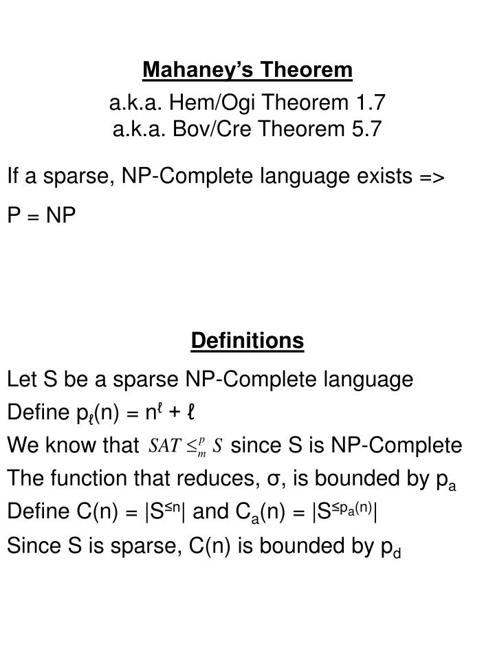
Mahaney’s Theorem a.k.a. Hem/Ogi Theorem 1.7 a.k.a. Bov/Cre Theorem 5.7 If a sparse, NP-Complete language exists => P = NP Definitions Let S be a sparse NP-Complete language Define pℓ(n) = nℓ + ℓ We know that since S is NP-Complete The function that reduces, σ, is bounded by pa Define C(n) = |S≤n| and Ca(n) = |S≤pa(n)| Since S is sparse, C(n) is bounded by pd

What did the sparse set say to its complement? “Why do you have to be so dense?” What we would want to happen, or Why this proof isn’t really easy What if S were in NP? Since S is NP-Complete, Since many-one reductions are closed under complementation, Thus, S is NP-Complete, S is co-NP-Complete and Hem/Ogi theorem 1.4 shows that P=NP. If only the proof were as easy as putting many-one reductions into a presentation…

Sorry, not quite so easy… However, S is not necessarily in NP Let’s define S in terms of Ca(n): S={x | y1, y2,…,yCa(|x|) [[(|y1|≤pa(|x|) ^ y1≠x ^ y1S] ^ [(|y2|≤pa(|x|) ^ y2≠x ^ y2S] ^ … … … ^ [(|yCa(|x|)|≤pa(|x|) ^ yCa(|x|)≠x ^ yCa(|x|)S] ^ all the y’s are distinct ] } S is for losers anyway… Hey, what about me? S≤pa(|x|) x y5 y2 y4 y1 y3

If only we had a way to have S be an NP language… Unfortunately, we cannot find the value of Ca(|x|) Fix this by parameterizing the number of y’s: S={<x,m>| y1, y2,…,ym [ [(|y1|≤pa(|x|)^y1≠x^y1S] ^ [(|y2|≤pa(|x|)^y2≠x^y2S] ^ … … … ^ [(|ym|≤pa(|x|) ^ ym≠x ^ ymS] ^ all the y’s are distinct ] } We will call this the pseudo-complement of S Note that for any <x,m>, <x,m> S iff: • m < Ca(|x|) or • m = Ca(|x|) and xS

How can this pseudo-complement help? We can prove that S is in NP by constructing an algorithm that decides S in non-deterministic polynomial time. Here’s a modified version of Bov-Cre’s algorithm: begin {input: x, m} if m > pd(pa(|x|)) then reject; guess y1, y2, …, ymin set of m-tuples of distinct words, each of which is of length, at most, pa(|x|); for i = 1 to m do if yi = x then reject; simulate MS(yi) along all Ms’s paths starting at i = 1 if Ms(yi) is going to accept and i < m simulate Ms(yi+1) along all Ms’s paths; if Ms(yi) is going to accept and i = m accept along that path; accept; end. Since S is in NP and S is NP-Complete, by some function ψ with bound pg

Why is it called recap? We never capped anything in the first place… capitulate \Ca*pit"u*late\, v. t. To surrender or transfer, as an army or a fortress, on certain conditions. [R.] So far, we’ve figured out the following: a) S many-one poly-time reduces to S by ψ with time bound pg b) SAT many-one poly-time reduces to S by σ with time bound pa c) The sparseness of S, C(n), is assured by pd d) Bov-Cre is way too algorithmic e) It is probably going to snow today --Hey, we all chose Rochester for some reason Next: What’s our favorite way to show P=NP? What’s our favorite way to show that SAT can be decided in polynomial time?

Get out the hedge trimmers… We have some formula F We want to know if it’s in SAT F F(v1=true) F(v1=false) . . . . . . Look familiar? This tree will get way too bushy for our purposes though, so we need to come up with a way to prune it

What’s this? A polynomial number of hedge trimmers? Only a theorist would think of something like that Given a formula, for each m in [1, pd(pa(|F|))] (this is every possible value of m for F) Create and prune a tree of assignments to variables just as we did for theorem 1.4 using a new pruning algorithm. When we get to the end, check each assignment to see if it’s satisfiable. • What we want to happen: • The number of leaves to be bounded by a polynomial • The pruning algorithm to be polynomial time • If F is satisfiable, then one of the leaves of the tree at the end is satisfiable • The snow to wait at least another 3-4 weeks so it wont instantly turn into slush and then ice • What that will get us: • A polynomial time algorithm that decides SAT • More time to put off getting snow tires for our cars

This slide is a great example of why I am not a digital art major For each stage of the tree: D is the set of all formulas generated by assigning true and false to the previous stage’s result D’ is the set of all formulas that have not been pruned from D (i.e. D’  D) F . . . . . . . . f . . . . . . . . . . How do we get to D’ from D? foreach f in D if |D’| ≤ pd(pg(pa(|F|))) and for eachf’ in D’ ψ(<σ(f), m>) ≠ψ(<σ(f’), m>) then add f to D’

When we’re done: Check each (variable-free) formula in the bottom layer to see if it’s satisfiable There are only a polynomial number If any is satisfiable, we’re done If for all m’s, no formula in the bottom layer is satisfiable, F is not satisfiable What’s next? Mappings… A few comparisons… Some polynomial bounds… Tree pruning… P=NP

Wait… I don’t get it… How is it so hard to draw nice trees when you are using presentation software with the “snap-to-grid” feature? Demystification (why the pruning works): It is important to note that when we have found the correct m = Ca(pa(|F|)) that f is not satisfiable iff ψ(<σ(f), Ca(pa(|F|))>) S Why, you ask? Recall that SAT reduces to S This f  SAT iff σ(f)  S Remember S? m=Ca(pa(|F|)) and σ(f)S iff <σ(f), Ca(pa(|F|))>S But S reduces to S too! <σ(f), Ca(pa(|F|))>S iff ψ(<σ(f), Ca(pa(|F|))>)S

If pa(pq(pr(pl(m+Cn(x))))) = pj(pn(p4(pa(nm – |1|)))), then 2 = 3 At least something is obvious in these slides… How does this help? There are a bounded number of unsatisfiable formulas that are mapped in S. This is pd (the sparsity of S) composed with pg (the limit on mappings to S through ψ) composed with pa (the limit on mappings to S through σ)* If we have chosen m = Ca(pa(|F|)), and we have found more than pd(pg(pa(|F|))) values then: Not all those ψ(<σ(f), m>)’s are in S so at least one of the f’s is satisfiable Thus, we can happily prune away all but one over the bound of these values, leaving a polynomial number while still guaranteeing one of them is sure to have a satisfying assignment. *Since m is constant for each tree, pairing σ(f) with m will not make the number of possible mappings in S bigger. Thus we don’t need to worry about the pairing in S changing the bound.

This complicated diagram makes it much easier to see. Trust me. SAT f f f pa(|f|) S r r r pa(|f|) S <r, m> <r, m> <r, m> pg(pa(|f|)) S Don’t forget that I’m sparse! t t t

Wait, if I prove P=NP, I win a million dollars… In the universe that has a sparse NP-Complete set, I am rich! Most of you are saying right now: “Yes, that is true, but how do you know if you have an m = Ca(pa(|F|))” An interesting fact: There are a polynomial number of m’s. Does it really matter what happens to the tree with m ≠ Ca(pa(|F|))? As long as we’re not wasting too much time pruning trees the wrong way, the other m’s don’t create too much overhead. If F is not satisfiable, we’ll never get a satisfying assignment; if F is satisfiable, maybe we’ll randomly keep an assignment with m≠Ca(pa(|F|)) but when m = Ca(pa(|F|)) each stage is guaranteed to have at least one satisfiable formula.

It all comes down to… wait, what were we talking about? Wait… did we just do what I think we did? Since for some value m, there is a tree that outputs a satisfiable formula iff the formula is satisfiable There are at most a polynomial number of leaves The pruning function runs in a polynomial amount of time There are only a polynomial number of trees We just decided if a formula is satisfiable in a polynomial amount of time Thus an NP-Complete language is decidable by a deterministic polynomial algorithm and P = NP …now what?

If a sparse, NP-Complete language exists => P = NP