Download
1 / 72
930 likes | 1.31k Views
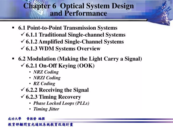
Chapter 6 Optical System Design and Performance. 6.1 Point-to-Point Transmission Systems 6.1.1 Traditional Single-channel Systems 6.1.2 Amplified Single-Channel Systems 6.1.3 WDM Systems Overview 6.2 Modulation (Making the Light Carry a Signal) 6.2.1 On-Off Keying (OOK) NRZ Coding

E N D
Chapter 6 Optical System Design and Performance • 6.1 Point-to-Point Transmission Systems • 6.1.1 Traditional Single-channel Systems • 6.1.2 Amplified Single-Channel Systems • 6.1.3 WDM Systems Overview • 6.2 Modulation (Making the Light Carry a Signal) • 6.2.1 On-Off Keying (OOK) • NRZ Coding • NRZI Coding • RZ Coding • 6.2.2 Receiving the Signal • 6.2.3 Timing Recovery • Phase Locked Loops (PLLs) • Timing Jitter
6.2.4 Analogue Amplitude Modulation • 6.2.5 Frequency Shift Keying (FSK) • 6.2.6 Phase Shift Keying (PSK) • 6.2.7 Polarity Modulation (PolSK) • 6.3 Transmission System Limits and Characteristics • 6.4 Optical System Engineering • 6.4.1 System Power Budgeting • Connector/Splice Loss Budgeting • Power Penalties • 6.4.2 Reflections • 6.4.3 Bit Error Rates (BER)
6.5 Optical Network • 6.6.1 Optical Networking Technologies • SONET • Gigabit Ethernet • Fiber Channel • ESCON • FDDL • 6.6.2 PON (Passive Optical Network)
6.1.1 Traditional Single-channel Systems 6.1 Point-to-Point Transmission Systems • A large number of electronic (digital) signals are combined using time division multiplexing (TDM) and presented to the optical transmission system as a single data stream. Figure 6.1 Conventional Long Distance Fiber Transmission System.
6.1.1 Traditional Single-Channel System • This single data stream is carried in an optical channel at speeds ranging from 155 Mbps to 1.2 Gbps. • The wavelength used is almost always 1310 nm. • Every 30-50 km the signal is received at a repeater station, converted to electronic form, re-clocked and re-transmitted. • When such a system needs to be upgraded all of the equipment in the link must be replaced. This is because the repeaters are code and speed sensitive devices.
6.1.1 Traditional Single-Channel System 6.1.1.1 Repeaters • What we do is extract the digital information stream from the old signal and then build a new signal containing the original information. This function is performed by a repeater. • As it travels along a wire, any signal (electrical or optical) is changed (distorted) by the conditions it encounters along its path. It also becomes weaker (attenuated) over distance due to energy loss. Thus it becomes necessary to boost the signal.
6.1.1 Traditional Single-Channel System • The signal can be boosted by simply amplifying it. This makes the signal stronger, but (as is shown in Figure 6.2) it amplifies a distorted signal. • A digital signal is received and it is reconstructed in the repeater. A new signal is passed on (the 2nd example of Figure 6.2) which is completely free from any distortion that was present when the signal was received at the repeater. Figure 6.2 Repeater Function compared with Amplification.
6.1.2 Amplified Single-Channel Systems Figure 6.3 Amplified Single-Channel Transmission System. The systems use optical amplifiers (EDFAs) with span lengths from 110 to 150 km.
6.1.2 Amplified Single-Channel Systems • The wavelength used is now 1550nm. This is done for two reasons: 1. To exploit the low attenuation window of fiber in the 1500 nm "window“. 2. To allow the use of Erbium Doped Fiber Amplifiers (EDFAs). • The distance between amplifiers is now increased to between 110 and 150 km. • The speed is generally increased to either 1.2 Gbps or 2.4 Gbps.
6.1.2 Amplified Single-Channel Systems • There are three significant changes: (compare to Fig. 6.3) 1.In older systems, the fiber didn't disperse the signal by very much because we were using the 1310 nm band. However, by moving to the 1550 nm band, we have brought on a dispersion problem. 2. The link may be upgraded to use higher speeds and the modulation format may be changed without changing equipment in the field. You only have to change the equipment at each end! 3. Provided the link has been planned properly it can now be upgraded to use WDM technology again without change to the outside plant.
6.1.2 Amplified Single-Channel Systems • EDFAs do produce some spontaneous emission noise and this tends to get amplified along the way (it is called ASE for Amplified Spontaneous Emission). • The amplified systems are considered significantly better than the earlier systems for the following reasons: 1. Amplifiers cost less than repeaters and require less maintenance. 2. The use of an amplifier enables future upgrades and changes to take place with minimal impact (read cost) on the installed link. 3. The use of the amplifier allows for future use of WDM technology with minimal change to the outside plant.
6.1.3 WDM Systems Overview • Figure 6.4 shows a typical first generation long distance WDM configuration. • Transmission is point-to-point. Figure 6.4 WDM Long Distance Fiber Transmission System.
6.1.3 WDM Systems Overview • It should be noted that each optical channel is completely independent of the other optical channels. It may run at its own rate (speed) and use its own encodings and protocols without any dependence on the other channels at all. • All of the current systems use a range of wavelengths between 1540 nm and 1560 nm. • There are two reasons for this: 1). to take advantage of the "low loss" transmission window in optical fiber; 2). to enable the use of erbium-dopped fiber amplifiers.
6.2 Modulation (Making the Light Carry a Signal) 6.2.1 On-Off Keying (OOK) • Most current optical transmission systems encode the signal as a sequence of light pulses in a binary form. This is called "on-off keying" (OOK). • It is like a very simple form of digital baseband transmission in the electronic world. • The signal is there or it isn't; beyond this the amplitude of the signal doesn't matter.
Non-Return to Zero (NRZ) Coding Figure 6.6. NRZ Coding • NRZ coding: A one bit is represented as the presence of light and a zero bit is represented as the absence of light. • This method of coding is used for some very slow speed optical links but has been replaced by other methods for most purposes.
NRZI Coding • In order to ensure enough transitions in the data for the receiver to operate stably, Most digital communication systems using fiber optics use Non-Return to Zero Inverted (NRZI) coding. • In NRZI coding, a zero bit is represented as a change of state on the line and a one bit as the absence of a change of state. This algorithm will obviously ensure that strings of zero bits do not cause a problem. Figure 6.6 NRZI Encoding Example
Return to Zero (RZ) Coding • In RZ coding the signal returns to the zero state every bit time. As illustrated a "1"bit is represented by a "ON" laser state for only half a bit time. Even in the "1" state the bit is "0" for half of the time. Figure 6.7 Return-to-Zero (RZ) Coding
Return to Zero (RZ) Coding • In a restricted bandwidth environment (such as in most electronic communications) this is not a coding of choice. The reason is that there are two different line states required to represent a bit (at least for a "1" bit). • In the optical fiber environment, bandwidth is not a major constraint. RZ coding is proposed as a basis for some Optical Time-Division Multiplexing (OTDM) systems.
6.2.2 Receiving the Signal 1. The incoming optical signal is converted to an electronic one using either a PIN-diode or an APD. 2. The signal is then pre-amplified and passed through a band-pass filter. There are a number of very low frequencies that get into the signal and there will be very high frequency harmonics that we don't need. Figure 6.8 Digital Receiver Functions.
6.2.2 Receiving the Signal 3. Further amplification with feedback control of the gain is used to provide stable signal levels for the rest of the process. This control circuit usually controls the bias current and thus the sensitivity of the photodiode as well. 4. A phase-locked loop is then used to recover a bit stream and (optionally) the timing information. 6. At this stage the stream of bits needs to be decoded from the coding used on the line into its data format coding. This process varies depending on the encoding and is occasionally integrated with the PLL depending on the code in use.
6.2.2 Receiving the Signal The important issues for the receiver are: • Noise:In the receiver we typically have a very low level input signal which requires a high gain and therefore we have the potential of high noise. Most of the noise in an unamplified optical link originates in the receiver. • Decision Point:The signal level at which we say that "all voltages below this will be interpreted as a 0 and all voltages above this will be interpreted as a 1". This is a critical parameter and must be determined dynamically. • Filtering:There are both low frequency (1000 Hz or so) and very high frequency components here that are not needed. These components both add to the noise and can cause malfunction of later stages in the process. Unwanted harmonics cause the PLL to detect false conditions (called "aliases").
6.2.3 Timing Recovery • There are many situations where a receiver needs to recover a very precise timing from the received bit stream in addition to just reconstructing the bit stream. • In order to recover precise timing not only must there be a good coding structure with many transitions, but the receiver must use a much more sophisticated device than a DPLL to recover the timing. This device is an analogue phase locked loop.
Phase Locked Loops (PLLs) • While DPLLs have a great advantage in simplicity and cost they suffer from three major deficiencies: 1. Even at quite slow speeds they cannot recover a good enough quality clocking signal for most applications where timing recovery is important. 2. As link speed is increased, they become less and less effective. Because circuit speeds have not increased in the same ratio as have communication speeds. 3. As digital signals increase in speed, they start behaving more like waveforms and less like "square waves" and the simplistic DPLL technique becomes less appropriate.
Phase Locked Loops (PLLs) What is needed is a continuous-time, analogue PLL that is illustrated in Figure 6.9. Figure 6.9 Operating Principle of a Continuous (Analogue) PLL
Phase Locked Loops (PLLs) • The VCO (Voltage Controlled Oscillator) is the key to the operation. 1. The VCO is designed to produce a clock frequency close to the frequency being received. 2. Output of the VCO is fed to a comparison device (a phase detector) which matches the input signal to the VCO output. 3. The phase detector produces a voltage output which represents the difference between the input signal and the output signal. 4. The voltage output is then used to control (change) the frequency of the VCO.
Phase Locked Loops (PLLs) • Properly designed, the output signal will be very close indeed to the timing and phase of the input signal. • There are two uses for the PLL output: 1. Recovering the bit stream (that is, providing the necessary timing to determine where one bit starts and another one ends). 2. Recovering the (average) timing (that is, providing a stable timing source at exactly the same rate as the timing of the input bit stream).
Timing Jitter • Jitter is the generic term given to the difference between the (notional) "correct" timing of a received bit and the timing as detected by the PLL. • Some bits will be detected slightly early and others slightly late. This means that the detected timing will vary more or less randomly by a small amount either side of the correct timing - hence the name "jitter". • Jitter is minimized if both the received signal and the PLL are of high quality. But although you can minimize jitter, you can never quite get rid of it altogether. • Jitter can have many sources. In an optical system the predominant cause of jitter is dispersion.
6.2.4 Analogue Amplitude Modulation (Continuous Wave) • Lasers have traditionally been very difficult to modulate using standard amplitude modulation. • This is caused by the non-linear response typical of standard Fabry-Perot lasers. • However, some DFB and DBR lasers have a reasonably linear response and can be modulated with an analogue waveform.
6.2.4 Analogue Amplitude Modulation (Continuous Wave) • The major current use of this is in cable TV and HFC distribution systems. An analogue signal is prepared exactly as though it was to be put straight onto the coaxial cable. Instead of putting it straight onto the cable it is used to modulate a laser. • At the receiver (often a simple PIN diode) the signal is amplified electronically and placed straight onto a section of coaxial cable. In standard (one-way) cable systems the maximum frequency present in the combined waveform is 500 MHz. In HFC systems this can increase up to 800 MHz or even 1 GHz.
6.2.5Frequency Shift Keying (FSK) • It is difficult to modulate the frequency of a laser and this is one of the reasons that FM optical systems are not yet in general use. However, Distributed Bragg Reflector (DBR) lasers are becoming commercially available. • For FSK (or any system using coherent detection) to work, the real problem is the need for coherent detection. • The receiver "locks on" to the signal and is able to detect signals many times lower in amplitude than simple detectors can use. This translates to greater distances between repeaters and lower-cost systems. • In addition, FSK promises much higher data rates than the pulse systems currently in use.
6.2.6 Phase Shift Keying (PSK) • You can't control the phase of a laser's output signal directly and so you can't get a laser to produce phase-modulated light. • However, a signal can be modulated in phase by placing' a modulation device in the light path between the laser and the fiber. • At this time PSK is being done in the laboratory but there are no available commercial devices. • Again, PSK requires coherent detection and this is difficult and expensive.
6.2.7 Polarity Modulation (PolSK) • Lasers produce linearly polarized light. Another modulation dimension can be achieved by introducing polarization changes. • Unfortunately, this is not an available technique (not even in the lab) but feasibility studies are being undertaken to determine if PolSK could be productively used for fiber communications.
6.3 Transmission System Limits and Characteristics The characteristics of various transmission systems are summarized in Table 6.1.
6.3 Transmission System Limits and Characteristics • A universally accepted measure of the capability of a transmission technology is the product of the maximum distance between repeaters and the speed of transmission. • In electrical systems, maximum achievable speed multiplied by the maximum distance at this speed yields a good rule of thumb constant. It is not quite so constant in optical systems, but nevertheless the speed and distance product is a useful guide to the capability of a technology. • Note that the Table 1 refers to single channel systems only.
6.3 Transmission System Limits and Characteristics Table 6.2 shows the attenuation characteristics of various transmission media and the maximum spacing of repeaters available on that medium.
6.3 Transmission System Limits and Characteristics • The concept of Table 6.2 is very conceptual. Special coaxial cable systems exist with repeater spacing of 12 km. • There exist systems capable of operating at very high speed (a few Mbps) over telephone twisted pairs for distances of four to six kilometers without repeaters. • The technology here is called ADSL (Asymmetric Digital Subscriber Line) or VDSL (Very fast Digital Subscriber Line). • This technology makes use of very sophisticated digital signal processing to eke the last bit per second from a very difficult medium. Nevertheless, the advantage of fiber transmission is obvious.
6.4 Optical System Engineering 6.4.1 System Power Budgeting • Attenuation of both multimode and single-mode fiber is generally linear with distance. The amount of signal loss due to cable attenuation is just the attenuation per kilometer multiplied by the distance. • To determine the maximum distance you can send a signal (leaving out the effects of dispersion), all you need to do is to add up all the sources of attenuation along the way and then compare it with the "link budget". • The link budget is the difference between the transmitter power and the sensitivity of the receiver.
6.4.1 System Power Budgeting • Thus, if you have a transmitter of power -10 dBm and a receiver that requires a signal of power -20 dBm (minimum) then you have 10 dB of link budget : 1. 10 connectors at 0.3 dB per connector = 3 dB 2. 2 km of cable at 2 dB/km (Multimode Graded index fiber at 1300 nm) = 4 dB 3. Contingency of (say) 2 dB for deterioration due to ageing over the life of the system. • This leaves us with a total of 9 dB system loss. This is within our link budget and so we would expect such a system to have sufficient power.
6.4.1 System Power Budgeting Figure 6.10 shows the characteristics of some typical devices versus the transmission speed (in bits/second).
6.4.1 System Power Budgeting 1. Every laser has a limit to the maximum speed at which it can be modulated but up to that limit power output is relatively constant. 2. LEDs produce less and less output as the modulation rate is increased. The difference in fiber types only relates to the amount of power you can couple from an LED into the different types of fiber. 3. All receivers require higher power as the speed is increased. To reliably detect a bit a receiver needs a certain number of photons. Therefore every time we double the modulation speed we need to also double the required power for a constant signal-to-noise ratio.
6.4.1 System Power Budgeting • If you look in the figure for a given bit rate (vertical line) there will be a difference between the required receiver power and the available transmitter power. • This difference is the amount we have available for losses in the fiber and connectors (and other optical devices such as splitters and circulators). • It is also very important to allow some margin in the design for ageing of components (lasers produce less power as they age, detectors become less sensitive, etc.).
Connector/Splice Loss Budgeting • Thesignal loss experienced at a connector or splice is not a fixed or predictable amount! The problem is the measured losses in actual splices and actual connectors vary considerably from each other. • Thegood news is that actual measurements form (roughly) a "normal" statistical distribution about the mean (average). • Table6.3 shows "typical" losses that may be expected from different connector types.
Connector/Splice Loss Budgeting • For a connection using almost any modern single-mode connector where both connectors are from the same supplier you can expect a mean loss of 0.2 dB with a standard deviation of 0.15 dB. 2. If the manufacturers of the two connectors are different, then you can expect an average loss of 0.35 dB with a standard deviation of 0.25 dB. 3. One type of single-mode connector may have an "average loss" of 0.2 dB but in practical situations this loss might vary from perhaps 0.1 dB to 0.8 dB.
Connector/Splice Loss Budgeting • If you know the average loss for a single connector and the standard deviation (s) of the connector loss for a particular situation then you can calculate these figures for any given combination. 1. The average (mean) of the total is just the average loss of a single connector multiplied by the number of connectors. 2. The standard deviation (s) of the total is just the standard deviation of a single connector multiplied by the square root of the number of connectors involved.
Connector/Splice Loss Budgeting • In long distance links it is common to regard splices as part of the fiber loss. So you might get raw SM fiber with a loss (at 1550 nm) of 0.21 dB/km. After cabling, this will increase to perhaps 0.23 dB/km. • For loss budget purposes you might allocate .26 dB/km for installed cable. Cable is typically supplied in 2 km lengths so in a100 km link there will be a minimum of 50 splices. • In the 1310 nm band, a typical cable attenuation might be 0.36 dB/km but it is typical to allocate 0.4 dB/km for fiber losses in new fiber used in this wavelength band. • The same piece of installed fiber cable would be budgeted at 0.4 dB/km when used in the 1310 nm band and at 0.26 dB/km when used in the 1550 nm band.
Power Penalties • There are a number of phenomena that occur within an optical transmission system that can be compensated for by increasing the power budget. • In each case the amount of additional power required to overcome the problem is termed the "power penalty". • The three most important issues here for digital systems are : 1. System noise 2. Effect of dispersion and 3. Extinction ratio
Power Penalties Signal-to-Noise Ratio (SNR) • The quality of any received signal in any communication system is largely determined by the ratio of the signal power to the noise power - the SNR. • In simple systems most of the noise comes from within the receiver itself and so is usually compensated for by an adjustment of the receiver sensitivity specification. • In complex systems with EDFAs, ASE noise becomes important and to compensate we indulge in power level planning throughout the system.
Power Penalties Inter-Symbol Interference (ISI) • Dispersion causes bits (really line states or bauds) to merge into one another on the link. • We can compensate for this by increasing the signal power level. • Thus for certain levels of dispersion we can nominate a system power budget (allowance) to compensate.
Power Penalties Extinction Ratio • If a zero bit is represented by a finite power level rather than a true complete absence of power then the difference between the power level of a 1-bit and that of a 0-bit is narrowed. • The power level of the 0-bit becomes the noise floor of every 1-bit. The receiver decision point has to be higher and therefore there is an increased probability of error. • This can be compensated for by an increase in available power level at the receiver. An extinction ratio of 10 dB incurs a power penalty (in either a PIN-diode receiver or an APD) of about 1 dB over what it would have been with a truly zero value for a 0-bit. • An extinction ratio of 3 dB causes a power penalty of 5 dB in a PIN-diode receiver and 7 dB in an APD.