Download
1 / 36
360 likes | 470 Views
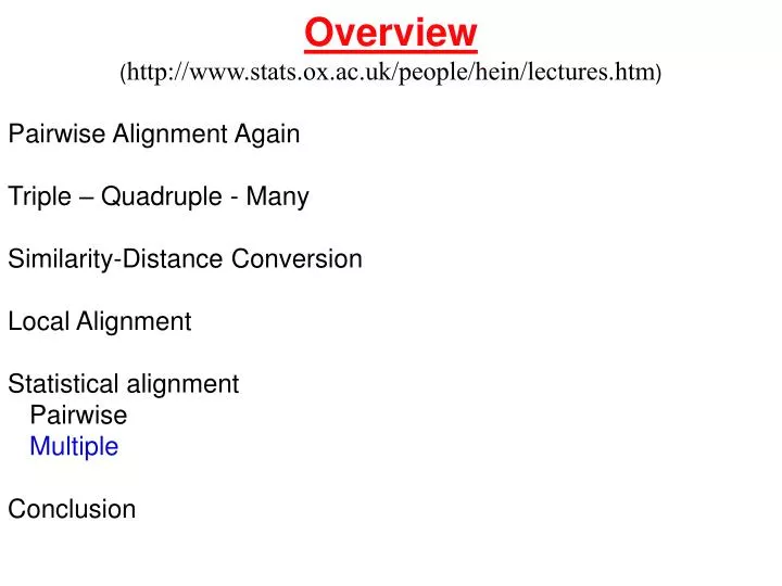
Overview ( http://www.stats.ox.ac.uk/people/hein/lectures.htm ) Pairwise Alignment Again Triple – Quadruple - Many Similarity-Distance Conversion Local Alignment Statistical alignment Pairwise Multiple Conclusion. Approaches to Data Analysis. s 1. s 2. s 3. s 4.

E N D
Overview (http://www.stats.ox.ac.uk/people/hein/lectures.htm) Pairwise Alignment Again Triple – Quadruple - Many Similarity-Distance Conversion Local Alignment Statistical alignment Pairwise Multiple Conclusion
Approaches to Data Analysis s1 s2 s3 s4 Data {GTCAT,GTTGGT,GTCA,CTCA} Parsimony, similarity, optimisation. GT-CAT GTTGGT GT-CA- CT-CA- statistics statistics Ideal Practice: 1 phase analysis. Actual Practice: 2 phase analysis.
Parsimony Alignment of two strings. Sequences: s1=CTAGG s2=TTGT. Basic operations: transitions 2 (C-T & A-G), transversions 5, indels (g) 10. {CTA,TT}AL + GG {CTAG,TTG}AL = {CTA,TTG}AL + G- {CTAG,TT}AL + -G Initial condition: D0,0=0. (Di,j = D(s1[1:i], s2[1:j])) Di,j=min { Di-1,j-1 + d(s1[i],s2[j]), Di,j-1 + g, Di-1,j +g} DCTA,TT + w(GG) =12 + 0 = 12 D4,3=DCTAG,TTG=min{DCTA,TTG + w(G-) = 4 + 10 = 14} DCTAG,TT + w(-G) = 22 + 10 = 32
40 32 22 14 9 17 T / 30 22 12 4 12 22 G / 20 12 2-12 22 32 T / 10 2 10 20 30 40 T / 0 10 20 30 40 50 C T A G G CTAGG Alignment: i v Cost 17 TT-GT
Alignment of three sequences. s1=ATCG s2=ATGCC s3=CTCC Alignment: AT-CG ATGCC CT-CC Consensus sequence: ATCC Configurations in an alignment column: - - n n n - n - - n - n - n n - n - - - n n n - Recursion:Di,j,k = min{Di-i',j-j',k-k' + d(i,i',j,j',k,k')} Initial condition: D0,0,0 = 0. Running time: l1*l2*l3*(23-1) Memory requirement: l1*l2*l3 New phenomena: ancestral sequence. A C ? A
C G G C Parsimony Alignment of four sequences s1=ATCG s2=ATGCC s3=CTCC s4=ACGCG Alignment: AT-CG ATGCC CT-CC ACGCG Configurations in alignment columns: - - - n - - - n n n - n n n n - - - n - n n - n - - n - n n n - - n - - n - n - n - n n - n n - n - - - - n n - - n n n n - n - Recursion: Di= min{Di-∆ + d(i,∆)} ∆ [{0,1}4\{0}4] Initial condition: D0 = 0. Computation time: l1*l2*l3*l4*24Memory : l1*l2*l3*l4
Alignment of many sequences. s1=ATCG, s2=ATGCC, ......., sn=ACGCG Alignment: AT-CG s1 s3 s4 ATGCC \ ! / ..... ---------- ..... / \ ACGCG s2 s5 Configurations in an alignment column: 2n-1 Recursion: Di=min{Di-∆ + d(i,∆)} ∆ [{0,1}n\{0}n] Initial condition: D0,0,..0 = 0. Computation time: ln*(2n-1)*n Memory requirement: ln (l:sequence length, n:number of sequences)
Fitch-Hartigan-Sankoff Algorithm (A,C,G,T) (9,7,7,7) / \ / \ Costs: Transition 2, / \ (A ,C,G, T) \ Transversion 5, indel 10. (10,2,10,2) \ / \ \ / \ \ / \ \ / \ \ / \ \ (A,C,G,T) (A,C,G,T) (A,C,G,T) * 0 * * * * * 0 * * 0 * Indel Constraint: Nucleotides is connected set.
Longer Indels TCATGGTACCGTTAGCGT GCA-----------GCAT gk : cost of indel of length k. Initial condition: D0,0=0 Di,j = min { Di-1,j-1 + d(s1[i],s2[j]), Di,j-1 + g1,Di,j-2 + g2,Di,j-3 + g3,, Di-1,j + g1,Di-2,j + g2,Di-3,j + g3,, } Cubic running time. Quadratic memory.
If gk = a + b*k, then quadratic running time. Gotoh (1982) Di,j is split into 3 types: 1. D0i,j as Di,j, except s1[i] must mactch s2[j]. 2. D1i,j as Di,j, except s1[i] is matched with "-". 3. D2i,j as Di,j, except s2[i] is matched with "-". Then:D0i,j = min(D0i-1,j-1, D1i-1,j-1, D2i-1,j-1) + d(s1[i],s2[j]) D1i,j = min(D1i,j-1 + b, D0i,j-1 + a + b) D2i,j = min(D2i-1,j + b, D0i-1,j + a + b) Comment: 1. Evolutionary Consistency Condition: gi + gj > gi+j
Distance-Similarity. (Smith-Waterman-Fitch,1982) Di,j=min{Di-1,j-1 + d(s1[i],s2[j]), Di,j-1 +g, Di-1,j +g} Si,j=max{Di-1,j-1 + s(s1[i],s2[j]), Si,j-1 -w, Si-1,j-w} Distance: Transitions:2 Transversions 5 Indels:10 M largest distance between two nucleotides (5). Similarity s(n1,n2) M - d(n1,n2) wk k/(2*M) + gk w 1/(2*M) + g Similarity Parameters: Transversions:0 Transitions:3 Identity:5 Indels: 10 + 1/10
40/-40.4 32/-27.3 22/-12.2 14/0.9 9/11.0 17/2.9 T 30/-30.3 22/-17.2 12/-2.1 4/11.0 12/2.9 22/-7.2 G 20/-20.2 12/-7.1 2/8.012/-2.1 22/-12.2 32/-22.3 T 10/-10.1 2/3.0 10/-7.1 20/-17.2 30/-27.3 40/-37.4 T 0/0 10/-10.1 20/-20.2 30/-30.3 40/-40.4 50/-50.5 C T A G G Comments 1. The Switch from Dist to Sim is highly analogous to Maximizing {-f(x)} instead of Minimizing {f(x)}. 2. Dist will based on a metric: i. d(x,x) =0, ii. d(x,y) >=0, iii. d(x,y) = d(y,x) & iv. d(x,z) + d(z,y) >= d(x,y). There are no analogous restrictions on Sim, giving it a larger parameter space.
Local alignment Smith,Waterman (1981 Global Alignment:Si,j=max{Di-1,j-1 + s(s1[i],s2[j]), Si,j-1 -w, Si-1,j-w} Local: Si,j=max{Di-1,j-1 + s(s1[i],s2[j]), Si,j-1 -w, Si-1,j-w,0} 0 1 0 .6 1 2 .6 1.6 1.6 3 2.6 Score Parameters: C 0 0 1 0 1 .3 .6 0.6 2 3 1.6 Match: 1 A 0 0 0 1.3 0 1 1 2 3.3 2 1.6 Mismatch -1/3 G / 0 0 .3 .3 1.3 1 2.3 2.3 2 .6 1.6 Gap 1 + k/3 C / 0 0 .6 1.6 .3 1.3 2.6 2.3 1 .6 1.6 GCC-UCG U / GCCAUUG 0 0 2 .6 .3 1.6 2.6 1.3 1 .6 1 A ! 0 1 .6 0 1 3 1.6 1.3 1 1.3 1.6 C / 0 1 0 0 2 1.3 .3 1 .3 2 .6 C / 0 0 0 1 .3 0 0 .6 1 0 0 G / 0 0 0 .6 1 0 0 0 1 1 2 U 0 0 1 .6 0 0 0 0 0 0 0 A 0 0 1 0 0 0 0 0 0 0 0 A 0 0 0 0 0 0 0 0 0 0 0 C A G C C U C G C U U
Progressive Alignment (Feng-Doolittle 1987 J.Mol.Evol.) Can align alignments and given a tree make a multiple alignment. * * alkmny-trwq acdeqrt akkmdyftrwq acdehrt kkkmemftrwq [ P(n,q) + P(n,h) + P(d,q) + P(d,h) + P(e,q) + P(e,h)]/6 * * *** * * * * * * Sodh atkavcvlkgdgpqvqgsinfeqkesdgpvkvwgsikglte-glhgfhvhqfg----ndtagct sagphfnp lsrk Sodb atkavcvlkgdgpqvqgtinfeak-gdtvkvwgsikglte—-glhgfhvhqfg----ndtagct sagphfnp lsrk Sodl atkavcvlkgdgpqvqgsinfeqkesdgpvkvwgsikglte-glhgfhvhqfg----ndtagct sagphfnp lsrk Sddm atkavcvlkgdgpqvq -infeak-gdtvkvwgsikglte—-glhgfhvhqfg----ndtagct sagphfnp lsrk Sdmz atkavcvlkgdgpqvq— infeqkesdgpvkvwgsikglte—glhgfhvhqfg----ndtagct sagphfnp Lsrk Sods vatkavcvlkgdgpqvq— infeak-gdtvkvwgsikgltepnglhgfhvhqfg----ndtagct sagphfnp lsrk Sdpb datkavcvlkgdgpqvq—-infeqkesdgpv----wgsikgltglhgfhvhqfgscasndtagctvlggssagphfnpehtnk sddm Sodb Sodl Sodh Sdmz sods Sdpb
*A # C G 0 # t # # # # Thorne-Kishino-Felsenstein Process l < m P(s) = (1-l/m)(l/m)l pA#A* .. * pT #T Time reversible
a t1 t2 s2 s1 t1 +t2 s1 s2 Time reversibility Pi,j(t) = probability that i has evolved into j after time t. p(i) = probability of i after infinitely long time - equilibrium distribution p(i) Pi,j(t) = p(j) Pj,i(t) t1-----------t2---------t3
Diff. Equations for p-functions # - - ... - # # # ... # Dpk = Dt*[l*(k-1) pk-1 + m*k*pk+1 - (l+m)*k*pk] # - - - ... - - # # # ... # Dp’k=Dt*[l*(k-1) p’k-1+m*(k+1)*p’k+1-(l+m)*k*p’k+m*pk+1] * - - - ... - * # # # ... # Dp’’k=Dt*[l*k*p’’k-1+m*(k-1)*p’’k+1-((k+1)l+mk)*p’’k] Initial Conditions: pk(0)= pk’’(0)= p’k (0)= 0 k>1 p0(0)= p0’’(0)= 1. p’0 (0)= 0
l & m into Alignment Blocks A. Amino Acids Ignored: # - - - # - - - - * - - - - ## # # - # # # # * # # # # k k k e-mt[1-lb(t)](lb(t))k-1 [1-e-mt-mb(t)][1-lb(t)](lb(t))k-1 [1-lb(t)](lb(t))k pk(t) p’k(t) p’’k(t) p’0(t)= mb(t) where b(t)=[1-e(l-m)t]/[m-l] B. AA Considered:T - - - RQ S W Pt(T-->R)*pQ*..*pW*p4(t) 4 T - - - - - R Q S WpR *pQ*..*pW*p’4(t) 4
Basic Pairwise Recursion (O(length3)) i j Survives Dies i-1 i-1 i i j-1 j j i-1 i-1 i i j-2 j j j-1
Fundamental Pairwise Recursion. P(s1i->s2j) = p’0P(s1i-1->s2j) + Initial Condition P(s10 ->s2j) = pj’’ps2[1:j] Simplification: Ri,j =(p1f(s1[i],s2[j]+p’1ps2j[j])P(s1i-1->s2j-1) P(s1i->s2j) = Ri,j + p’0 P(s1i->s2j-1) P(s1i->s2j) = p’0P(s1i-1->s2j)+ lbP(s1i->s2j-1) + (p1f(s1[i],s2[j]+p’1ps2j[j]- lb ps2j[j] ))P(s1i-1->s2j-1) Probability of observation P(s1 , s2) = P(s1) P(s1 ->s2)
a-globin (141) and b-globin (146) 430.108 : -log(a-globin) 327.320 : -log(a-globin b-globin) 730.428 : -log(l(sumalign)) l*t: 0.0371805 +/- 0.0135899 m*t: 0.0374396 +/- 0.0136846 s*t: 0.91701 +/- 0.119556 E(Length) E(Insertions,Deletions) E(Substitutions) 143.499 5.37255 131.59 Maximum contributing alignment: V-LSPADKTNVKAAWGKVGAHAGEYGAEALERMFLSFPTTKTYFPHF-DLS--H---GSAQVKGHGKKVADAL VHLTPEEKSAVTALWGKV--NVDEVGGEALGRLLVVYPWTQRFFESFGDLSTPDAVMGNPKVKAHGKKVLGAF TNAVAHVDDMPNALSALSDLHAHKLRVDPVNFKLLSHCLLVTLAAHLPAEFTPAVHASLDKFLASVSTVLTSKYR SDGLAHLDNLKGTFATLSELHCDKLHVDPENFRLLGNVLVCVLAHHFGKEFTPPVQAAYQKVVAGVANALAHKYH Ratio l(maxalign)/l(sumalign) = 0.00565064
Probability for substitution: = 0.46 #children: p p' p'': 0. 0.0 3.60 10-2 9.64 10-1 1. 9.28 10-1 6.30 10-4 3.45 10-2 2. 3.32 10-2 2.26 10-5 1.23 10-3 3. 1.19 10-3 8.10 10-7 4.43 10-5 4. 4.27 10-5 2.90 10-8 1.59 10-6 5. 1.53 10-6 1.04 10-9 5.70 10-8 b(t) = 9.64 * 10-1lb(t) = 3.46 * 10-2
Accelerations of pairwise algorithm 1 2 - Better numerical search 3 - Simpler recursion 4 - Better computers 1991->2000 : an 106 acceleration for 2 proteins 1500 long.
Homology Test Wi,j= -ln(pi*P2.5i,j/(pi*pj)) D(s1,s2) is evaluated in D(s1,s2*) Real s1 = ATWYFCAK-AC Random s1 = ATWYFC-AKAC s2 = ETWYKCALLAD s2* = LTAYKADCWLE *** ** * * * This test: 1. Test the competing hypothesis that 2 sequences are 2.5 events apart versus infinitely far apart. 2. It only handles substitutions “correctly”. The rationale for indel costs are more arbitrary. 3. It samples in (pi*pj) by permuting the order of amino acids in the second. I.e. uses drawing without replacement – a hypergeometric distribution.
Steel-Hein Algorithm *TTGT *ACGC s2 s1 a *###### s3 *ACGGT
Binary Tree Problem TGA ACCT s1 s3 a1 a2 s2 s4 GTT ACG
Generating Ancestral Sequences 1 Sequence # E * l/m 1- l/m #l/m 1- l/m 2 Sequence - # # E # # - E * * lb l/m (1- lb)e-m l/m (1- lb)(1- e-m) (1- l/m) (1- lb) - # lb l/m (1- lb)e-m l/m (1- lb)(1- e-m) (1- l/m) (1- lb) _ #lb l/m (1- lb)e-m l/m (1- lb)(1- e-m) (1- l/m) (1- lb) # - lb a1 * - # E a2 * # # E lb l/m (1- lb)e-m (1- l/m) (1- lb)
Fundamental Multiple Recursion I s1 - C G C T A s2 A G A A T T a1 #- a ---> e . . . . . . . a2 ## s3 A G C G G s4 G - C C T G # # # # - # = Sum over all String partitions - Anc. state survivals - Anc. state MC jumps
Fundamental Multiple Recursion II Pa(Sk): Epifixes (S1[k+1:l1]) starting in given MC starts i state a. Pa(Sk) = Where P(kS i,H ! ) = F(kSi,H)
Fundamental 4 sequence Recursion Not a proper recursion! Initialisation: PEE(Ø) =1 and Pa(Ø) are directly calculatable. O(l2k)shown, O(lk) Algorithm possible Toy 4-Sequence Program almost ready. This approach could analyse up to 6-7 sequences. Jens Ledet and others are working on Gibbs sampler approach.
Statistical Alignment Summary Motivation for statistical alignment: Data is sequences not alignment! Problems ahead: Longer Insertion Deletion Process Position Heterogeneous Process Simultaneous Comparative Gene Finding and Alignment. Making an TKF-process with a given HMM as stationary distribution. Explore non-TKF processes.