Download
1 / 54
610 likes | 976 Views
Game Playing. "Abstract" games are of interest to AI (artificial intelligence) because: Games states are accessible and easy to represent Games are usually restricted to a small number of well-defined actions Successful programs which play complex games are evidence of machine intelligence

E N D
Game Playing "Abstract" games are of interest to AI (artificial intelligence) because: • Games states are accessible and easy to represent • Games are usually restricted to a small number of well-defined actions • Successful programs which play complex games are evidence of machine intelligence Game playing goes beyond the search technique A* because of opponent behavior, which is unpredictable.
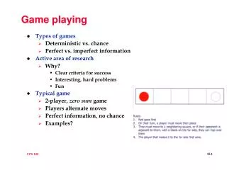
Games vs. Search Problems • “Unpredictable” opponent • Solution is a contingency plan • Time limits • Unlikely to find goal, must approximate • Plan of attack: • Algorithm for perfect play: Minimax • Finite horizon and evaluation functions • “Pruning” to reduce costs
Types of Games Deterministic Chance chess, checkers, go, othello backgammon, monopoly Perfect Information Imperfect Information battleship bridge, poker, scrabble, nuclear war
Two-Person Zero-Sum Games • A zero-sum game is one in which a gain by one player (MAX) is equivalent to a loss by the other (MIN), leading to a sum of zero overall advantage • A two-person game defines a state space that has the game's starting configuration as its root • Final states in the state space signify either a win for MAX, or a win for MIN, or a draw • MAX's goal: maximize the value of the final state. • MIN's goal: minimize the value of the final state
Formal Parts of a Game • Initial state, including whose move it is (either MAX or MIN) • Operators, defining the legal moves • Terminal test, determining when the game is over • Utility function, giving a numeric value to the outcome of a game: • A higher utility is a win for MAX; a lower utility is a win for MIN. • These parts define a game tree
Partial Game Tree for Tic-Tac-Toe MAX(X) MIN(O) MAX(X) MIN(O) Terminal utility Draw Win for MIN Win for MAX
One Version of the Game of Nim • Start with one pile of N objects, say coins • A move consists of dividing any pile into two unequal-size piles • The first player who cannot move loses
Partial Game Tree for Nim with N=7 7 6-1 5-2 4-3 5-1-1 4-2-1 4-2-1 3-2-2 4-2-1 3-3-1 Note that state 4-2-1 is repeated. We can simplify the structure by drawing a general graph.
Complete State Space for Nim (7) 7 MIN 6-1 5-2 4-3 MAX 5-1-1 4-2-1 3-2-2 3-3-1 MIN 4-1-1-1 3-2-1-1 2-2-2-1 MAX Win for MAX Win for MIN 3-1-1-1-1 2-2-1-1-1 MIN 2-1-1-1-1-1 MAX
A Forced Win for MAX (Bold Lines) 7 MIN 6-1 5-2 4-3 MAX 5-1-1 4-2-1 3-2-2 3-3-1 MIN 4-1-1-1 3-2-1-1 2-2-2-1 MAX 3-1-1-1-1 2-2-1-1-1 MIN 2-1-1-1-1-1 MAX If MIN goes first, and MAX plays intelligently, a win can be guaranteed for MAX
Game Tree Terminology • Each level in a game search tree is called a "ply". "2-ply" corresponds to a player's move and the opponent's response • Here is a trivial 2-ply tree:
Interpreting the Game Tree • MAX is to move first • MAX can choose among 3 actions A1, A2 and A3 • MIN can respond to move Ai with Ai1, Ai2, or Ai3 • There are 9 terminal states, whose utility values for MAX are computed and shown below the state • On the basis of the terminal utilities, the utilities of nonterminal states are "backed up" the tree to the root, indicating that MAX should choose A1 • How?
The Minimax Procedure for Simple Games • Generate entire game tree • Apply utility function to each terminal state • Determine utility of states at previous ply by asking, "If MIN had these choices at this ply, what would MIN choose?" (Answer: the minimum utility state) • At ply previous to THAT, determine utility by taking the maximum of the minimums taken by MIN • Continue in this way up the tree until root is reached
Exhaustive Minimax for Nim 1 7 MIN 1 1 1 6-1 5-2 4-3 MAX 1 0 0 1 5-1-1 4-2-1 3-2-2 3-3-1 MIN 0 1 0 4-1-1-1 3-2-1-1 2-2-2-1 MAX 0 1 3-1-1-1-1 2-2-1-1-1 terminal utility values for MAX MIN 0 0 0 0 2-1-1-1-1-1 MAX
A Forced Win for MAX (Bold Lines) 1 7 MIN 1 1 1 6-1 5-2 4-3 MAX 1 0 0 1 5-1-1 4-2-1 3-2-2 3-3-1 MIN 0 1 0 4-1-1-1 3-2-1-1 2-2-2-1 MAX 0 1 3-1-1-1-1 2-2-1-1-1 MIN 0 0 0 0 2-1-1-1-1-1 MAX If MIN goes first, and MAX plays intelligently, a win can be guaranteed for MAX
Implementing Minimax (Pseudocode) Suppose: Integer utility(State s); // returns a state's utility value State nextState(State s, Move m); // returns the new state // resulting from applying m to s Successors expand(State s); // returns all of the possible next states Move minimaxDecision(State s) for each Move m from s do value[m] = minimaxValue(nextState(s,m)) return the m with the highest value[m]
Implementing Minimax (cont'd) Integer minimaxValue(State s) if s is a terminal state then return utility(s) else successors = expand(s) if it is MAX's turn to move then return the highest minimaxValue of successors else return the lowest minimaxValue of successors
Recall Example Tree R X Y Z F G C D H I A B E
Trace of Minimax on Example Tree > minimaxDecision(R) > minimaxValue(X) > minimaxValue(A) => returns 3 > minimaxValue(B) => returns 12 > minimaxValue(C) => returns 8 < minimaxValue(X) => returns 3 [minimum value of 3, 12, and 8] > minimaxValue(Y) > minimaxValue(D) => returns 2 > minimaxValue(E) => returns 4 > minimaxValue(F) => returns 6 < minimaxValue(Y) => returns 2 [minimum value of 2, 4, and 6] > minimaxValue(Z) > minimaxValue(G) => returns 14 > minimaxValue(H) => returns 5 > minimaxValue(I) => returns 2 < minimaxValue(Z) => returns 2 [minimum value of 14, 5, and 2] < minimaxDecision(R) => returns A1 [the move that produces the state with the highest value in 3, 2, and 2]
Efficiency of Minimax The branching factorb of a game is the average number of possible moves from a state (3 in example). The number of calls to minimaxValue depends upon b and the depth N of the game tree: 32 + 3 = 12 b N can be ignored In general, the number of calls to minimaxValue is: O(bN)
Efficiency Comparisons O(bN) minimaxValue O(N) array implementation of priority queue time O(logN) binary heap implementation of priority queue N 0
Comparison of Big-O Rates of Growth N log2N N2 2N 1 0 1 2 2 1 4 4 4 2 16 16 8 3 64 256 16 4 256 65,536 32 5 1024 4,294,967,296 64 6 4096 5 years' worth of instructions on a supercomputer 128 7 16,384 600,000 times greater than age of universe in nanosecs
Properties of Minimax • Complete? That is, will it find a move given enough time? • Yes, if tree is finite • Optimal? That is, if there is a forced win, will it find it? • Yes, provided opponent is trying to win • Time complexity: O(bm) • Space complexity: O(bm) -- depth-first search • For chess, b 35, m 100 for reasonable games
When the Game Tree Cannot Be Exhaustively Searched • Alter minimax in two ways: • Replace the terminal test with a cutoff test, so only a subtree of the entire tree is searched. • Replace utility function with an evaluation function eval and apply it to the leaves of the subtree • Usually the cutoff is a fixed ply depth N determined by the available resources of time and memory • This strategy is called N-move lookahead
Minimax Modified Integer minimaxValue(State s) if s does not survive cutoff test then return eval(s) else successors = expand(s) if it is MAX's turn to move then return the highest minimaxValue of successors else return the lowest minimaxValue of successors
Evaluation Functions Somewhat like the 8-puzzle heuristic, an evaluation function estimates the utility of the game from a given (nonterminal) position. Chess example: Add up the "material values" of pieces: piece value pawn 1 bishop 3 knight 3 rook 5 queen 9 Other features such as "pawn structure" or "king safety" can be given values
Chess Board Evaluations white has better pawn structure
Weighted Linear Functions As Evaluation Functions Suppose: • there are n features to be included in the evaluation • f1, f2, . . . , fn are the number of pieces with each feature • w1,w2, . . . , wn are the weights associated with each feature Then the evaluation function can be computed by: w1f1 + w2f2 + . . . + wnfn
Problems with Search Cutoff • Arbitrary depth limit may fail to recognize an impending disaster: Suppose the lookahead stops at this point. White is ahead by a knight and thus has material advantage. But the eval function will not take into account that white's queen is about to be lost without compensation.
Problems with Search Cutoff (cont'd) • "Horizon problem": cutting off the search may fail to foresee a significant event that is inevitable: Black is slightly ahead in material, but when white advances pawn to the eighth row it becomes a queen. Black can be fooled into thinking the queening move can be avoided by checking white with the rook. If the lookahead is not far enough, the queening move will be pushed "over the horizon" of what can be predicted.
The Need for Game Tree Pruning • An ordinary computer can search about 1000 chess states per second • Tournament chess allows 150 seconds per move, so 150,000 states can be searched • The branching factor b of chess is about 35 Q: How many ply p can the computer look ahead? A: 35p = 150,000, so 3 < p < 4 Thus the computer can do a lookahead of 3 or 4 ply 4-ply: human novice 8-ply: human master, typical PC 12-ply: Kasparov, Deep Blue
Game Tree Pruning A full game tree:
Game Tree Pruning (cont'd) Depth cutoff This part of the tree is not examined
Game Tree Pruning (cont'd) Suppose you can determine that these states will never be reached
Game Tree Pruning (cont'd) Then all of their descendants can be ignored
Game Tree Pruning (cont'd) So the depth cutoff can be increased From here And these To here These nodes can be examined
- Pruning This technique recognizes when a game tree state can NEVER BE REACHED IN ACTUAL PLAY. R A B C After looking ahead to here, MAX knows that the utility for MIN of state B will be 2 or less. Since this cannot beat the utility already found for state A, MAX knows that B will not be chosen. So the rest of the subtree can be ignored (pruned).
- Pruning Example 3 Max 3 Min 3 12 8
- Pruning Example (cont'd) 3 Max 2 3 Min X X 2 3 12 8 These nodes do not need to be analyzed.
- Pruning Example (cont'd) 3 Max 2 3 14 Min X X 2 3 12 8 14
- Pruning Example (cont'd) 3 Max 14 5 2 3 Min X X 5 2 3 12 8 14
- Pruning Example (cont'd) 3 3 Max 14 5 2 2 3 Min X X 5 2 2 3 12 8 14
General - Principle If at node n a player has already noticed that a better choice existed at node m at some point further up the tree, then n will never be reached
Implementation of - Search • Similar to minimaxValue, only two mutually recursive functions are used: • maxValue is called when it is MAX's turn • minValue is called when it is MIN's turn • Since a depth-first search of the subtree is done, it is easy to pass along: • the best score for MAX so far along the current path () • the best score for MIN so far along the current path ()
- Implementation (cont'd) • is initialized to -∞ and only increases • is initialized to ∞ and only decreases • If ever becomes less than or equal to , the search (from the current node) is abandoned cutoff - Depth
Minimax Modified for - Pruning Move minimaxDecision(State s) global Integer = -∞ global Integer = ∞ for each Move m from s do value[m] = minimaxValue(nextState(s,m), , ) return the m with the highest value[m] Integer minimaxValue(State s, Integer , Integer ) if it is MAX's turn to move then return = maxValue(s, , ) else return = minValue(s, , )
- Implementation (cont'd) Integer maxValue(State s, Integer , Integer ) if s does not survive cutoff test thenreturn eval(s) foreach successor in expand(s) do = Maximum(, minValue(successor,,)) if<=thenreturn return Integer minValue(State s, Integer , Integer ) if s does not survive cutoff test thenreturn eval(s) foreach successor in expand(s) do = Minimum(, maxValue(successor,,)) if<=thenreturn return
Properties of - Search • Pruning does not affect final result • Good move ordering improves effectiveness of pruning • With “perfect ordering” time complexity = O(bm/2) • Doubles depth of search • Can reach depth 8 and play good chess
History of Chess Programs Chess ratings: 1000: beginning human, 2750: world champion • 1970: Early winners of ACM North American Computer Chess Championships were rated less than 2000, used: • - search • book openings • infallible endgame algorithms