Abstract

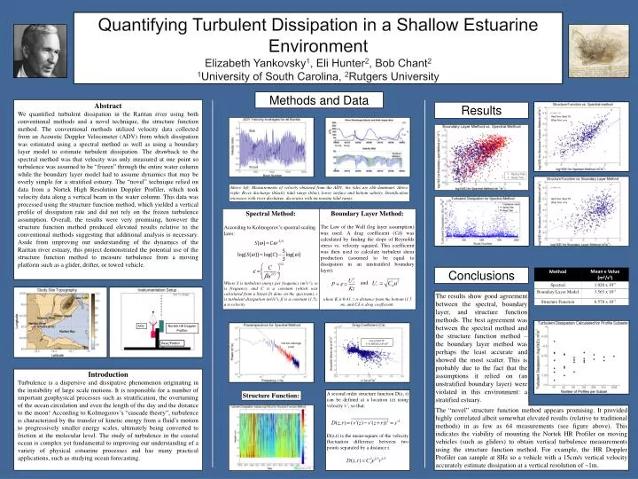
1. Quantifying Turbulent Dissipation in a Shallow Estuarine EnvironmentElizabeth Yankovsky1, Eli Hunter2, Bob Chant21University of South Carolina, 2Rutgers University Methods and Data Abstract We quantified turbulent dissipation in the Raritan river using both conventional methods and a novel technique, the structure function method. The conventional methods utilized velocity data collected from an Acoustic Doppler Velocimeter (ADV) from which dissipation was estimated using a spectral method as well as using a boundary layer model to estimate turbulent dissipation. The drawback to the spectral method was that velocity was only measured at one point so turbulence was assumed to be “frozen” through the entire water column while the boundary layer model had to assume dynamics that may be overly simple for a stratified estuary. The “novel” technique relied on data from a Nortek High Resolution Doppler Profiler, which took velocity data along a vertical beam in the water column. This data was processed using the structure function method, which yielded a vertical profile of dissipation rate and did not rely on the frozen turbulence assumption. Overall, the results were very promising, however the structure function method produced elevated results relative to the conventional methods suggesting that additional analysis is necessary. Aside from improving our understanding of the dynamics of the Raritan river estuary, this project demonstrated the potential use of the structure function method to measure turbulence from a moving platform such as a glider, drifter, or towed vehicle. Results Red line: Best fit Blue line: x=y Ebb Spring Neap Flood Above left: Measurements of velocity obtained from the ADV; the tides are ebb dominant. Above right: River discharge (black), tidal range (blue), lower surface and bottom salinity. Stratification increases with river discharge, decreases with increasing tidal range. Red line: Best fit Blue line: x=y Boundary Layer Method: The Law of the Wall (log layer assumption) was used. A drag coefficient (Cd) was calculated by finding the slope of Reynolds stress vs. velocity squared. This coefficient was then used to calculate turbulent shear production (assumed to be equal to dissipation in an unstratified boundary layer). and where K is 0.41, z is distance from the bottom (1.5 m), and Cd is drag coefficient. Spectral Method: According to Kolmogorov’s spectral scaling laws: Where S is turbulent energy per frequency (m2s-1), ω is frequency, and C is a constant (which was calculated from a linear fit done on the spectrum), ϵ is turbulent dissipation (m2/s3), β is a constant (1.5), u is velocity. Conclusions The results show good agreement between the spectral, boundary layer, and structure function methods. The best agreement was between the spectral method and the structure function method – the boundary layer method was perhaps the least accurate and showed the most scatter. This is probably due to the fact that the assumptions it relied on (an unstratified boundary layer) were violated in this environment: a stratified estuary. ADV Nortek HR Doppler Profiler Line of best fit: Y=-0.00032x-2.8*10-6 Base/Platform Inertial subrange (red) Introduction Turbulence is a dispersive and dissipative phenomenon originating in the instability of large scale motions. It is responsible for a number of important geophysical processes such as stratification, the overturning of the ocean circulation and even the length of the day and the distance to the moon! According to Kolmogorov’s “cascade theory”, turbulence is characterized by the transfer of kinetic energy from a fluid’s motion to progressively smaller energy scales, ultimately being converted to friction at the molecular level. The study of turbulence in the coastal ocean is complex yet fundamental to improving our understanding of a variety of physical estuarine processes and has many practical applications, such as studying ocean forecasting. A second order structure function D(z, r) can be defined at a location (z) using velocity v’, so that: D(z,r) is the mean-square of the velocity fluctuation difference between two points separated by a distance r. Structure Function: The “novel” structure function method appears promising. It provided highly correlated albeit somewhat elevated results (relative to traditional methods) in as few as 64 measurements (see figure above). This indicates the viability of mounting the Nortek HR Profiler on moving vehicles (such as gliders) to obtain vertical turbulence measurements using the structure function method.For example, the HR Doppler Profiler can sample at 8Hz so a vehicle with a 15cm/s vertical velocity accurately estimate dissipation at a vertical resolution of ~1m.