Proteins

1. SMA5233 Particle Methods and Molecular DynamicsLecture 5: Applications in Biomolecular Simulation and Drug Design A/P Chen Yu ZongTel: 6516-6877Email: phacyz@nus.edu.sghttp://bidd.nus.edu.sgRoom 08-14, level 8, S16 National University of Singapore

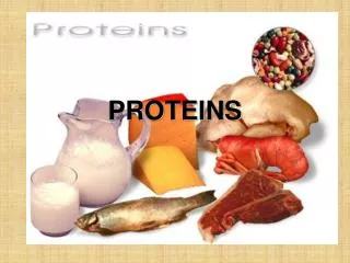
2. Proteins • Proteins are life’s machines, tools and structures • Many jobs, many shapes, many sizes

3. Proteins • Proteins are life’s machines, tools and structures • Nature reuses designs for similar jobs 1enh 1f43 1ftt 1bw5 1du6 1cqt 1hdd

4. Proteins • Proteins are hetero-polymers of specific sequence • There are 20 common polymeric units (amino acids) • Composed of a variety of basic chemical moieties • Chain lengths range from 40 amino acids on up MKLVDYAGE

5. Proteins • Proteins are hetero-polymers that adopt a unique fold MKLVDYAGE ?

6. Proteins • Protein folding as a reaction Transition state Bad Free Energy Reactants Products Good

7. Proteins • Protein folding … Transition state Bad Denatured / Partially Unfolded Free Energy Native Good

8. Proteins • Folded proteins Transition state Bad Denatured / Partially Unfolded Free Energy Native Folded, active, functional, biologically relevant state (ensemble of conformers) Good

9. Proteins • Folded proteins Transition state Bad Denatured / Partially Unfolded Free Energy Native Static, 3D coordinates of some proteins’ atoms are available from x-ray crystallography & NMR Good

10. Proteins • Folded proteins Transition state Bad Denatured / Partially Unfolded Free Energy Native Static, 3D coordinates of some proteins’ atoms are available from PDB http://www.pdb.org Good

11. Proteins • Folded proteins are complex and dynamic molecules Transition state Bad Denatured / Partially Unfolded Free Energy Native Good

12. Proteins • Folded proteins are complex and dynamic molecules Transition state Bad Denatured / Partially Unfolded Free Energy Native Good

13. Molecular Dynamics • MD provides atomic resolution of native dynamics PDB ID: 3chy, E. coli CheY 1.66 Å X-ray crystallography

14. Molecular Dynamics • MD provides atomic resolution of native dynamics PDB ID: 3chy, E. coli CheY 1.66 Å X-ray crystallography

15. Molecular Dynamics • MD provides atomic resolution of native dynamics 3chy, hydrogens added

16. Molecular Dynamics • MD provides atomic resolution of native dynamics 3chy, waters added (i.e. solvated)

17. Molecular Dynamics • MD provides atomic resolution of native dynamics 3chy, waters and hydrogens hidden

18. Molecular Dynamics • MD provides atomic resolution of native dynamics native state simulation of 3chy at 298 Kelvin, waters and hydrogens hidden

19. Proteins • Folding & unfolding at atomic resolution Transition state Bad Denatured / Partially Unfolded Free Energy Native Disordered, non-functional, heterogeneous ensemble of conformers Good

20. Proteins • Protein folding, why we care how it happens Transition state Denatured / Partially Unfolded Free Energy mutation Native mutation mutation Many diseases are related to protein folding and / or misfolding in response to genetic mutation.

21. Proteins • Protein folding, why we care how it happens Transition state Denatured / Partially Unfolded Free Energy mutation Native mutation mutation We need to comprehend folding to build nano-scale biomachines (that could produce energy, etc…)

22. Proteins • Protein folding takes > 10 μs (often much longer) Transition state Bad Denatured / Partially Unfolded Free Energy Native Good

23. Proteins • Protein folding takes > 10 μs (often much longer) Transition state Bad Denatured / Partially Unfolded Free Energy Native Good

24. Proteins • Protein folding is the reverse of protein unfolding Transition state Bad Denatured / Partially Unfolded Free Energy Native Good

25. Proteins • Protein unfolding is relatively invariant to temperature Transition state Bad Denatured / Partially Unfolded Native Free Energy Temperature Good

26. Molecular Dynamics • MD provides atomic resolution of folding / unfolding unfolding simulation (reversed) of 3chy at 498 Kelvin, waters & hydrogens hidden

27. Forces Involved in the Protein Folding • Electrostatic interactions • van der Waals interactions • Hydrogen bonds • Hydrophobic interactions(Hydrophobic molecules associate with each other in water solvent as if water molecules is the repellent to them. It is like oil/water separation. The presence of water is important for this interaction.)

28. O ＋ ー H Energy Functions used in Molecular Simulation Φ Θ r Dihedral term Bond stretching term Angle bending term The most time demanding part. Van der Waals term H-bonding term Electrostatic term r r r

29. System for MD Simulations Without water molecules With water molecules # of atoms: 304 # of atoms:　304 + 7,377 = 7,681

30. MD Requires Huge Computational Cost • Time step of MD (Δt) is limited up to about 1 fsec (10-15 sec).←The size of Δt should beapproximately one-tenth the time of the fastest motion in the system. For simulation of a protein, because bond stretching motions of light atoms (ex. O-H, C-H), whose periods are about 10-14 sec, are the fastest motions in the system for biomolecular simulations, Δt is usually set to about 1 fsec. • Huge number of water molecules have to be used in biomolecular MD simulations.← The number of atom-pairs evaluated for non-bonded interactions (van der Waals, electrostatic interactions) increases in order of N 2 (N is the number of atoms). It is difficult to simulate for long time. Usually a few tens of nanoseconds simulation is performed.

31. 10-3 10-9 100 10-15 10-12 10-6 (fs) (ns) (μs) (ps) (s) (ms) MD Time Scales of Protein Motions and MD Permeation of an ion in Porin channel Elastic vibrations of proteins α-Helix folding β-Hairpinfolding Bond stretching Protein folding Time It is still difficult to simulate a whole process of a protein folding using the conventional MD method.

32. Much Faster, Much Larger! • Special-purpose computer • Calculation of non-bonded interactions is performed using the special chip that is developed only for this purpose. • For example; • MDM (Molecular Dynamics Machine) or MD-Grape: RIKEN • MD Engine: Taisho Pharmaceutical Co., and Fuji Xerox Co. • Parallelization • A single job is divided into several smaller ones and they are calculated on multi CPUs simultaneously. • Today, almost MD programs for biomolecular simulations (ex. AMBER, CHARMm, GROMOS, NAMD, MARBLE, etc) can run on parallel computers.

33. Brownian Dynamics (BD) • The dynamic contributions of the solvent are incorporated as a dissipative random force (Einstein’s derivation on 1905). Therefore, water molecules are not treated explicitly. • Since BD algorithm is derived under the conditions that solvent damping is large and the inertial memory is lost in a very short time, longer time-steps can be used. • BD method is suitable for long time simulation.

34. System for BDSimulations Without water molecules With water molecules # of atoms: 304 # of atoms:　304 + 7,377 = 7,681

35. Algorithm of BD The Langevin equation can be expressed asHere, ri and mi represent the position and mass of atom i, respectively. ζi is a frictional coefficient and is determined by the Stokes’ law, that is, ζi = 6πaiStokesη in which aiStokes is a Stokes radius of atom i and η is the viscosity of water. Fi is the systematic force on atom i. Ri is a random force on atom i having a zero mean <Ri(t)> = 0 and a variance <Ri(t)Rj(t)> = 6ζikTδijδ(t); this derives from the effects of solvent. For the overdamped limit, we set the left of eq.7 to zero,The integrated equation of eq. 8 is called Brownian dynamics;where Δt is a time step and ωi is a random noise vector obtained from Gaussian distribution. (7) (8) (9)

36. Computational Time of BD Computational time required for 1 nsec simulation of a peptide †MTS(Multiple time step) algorithm:　This method reduces the frequency of calculation of the most time-demanding part （non-bonded energy terms）.

37. Folding Simulation of an α-Helical Peptide using BD 1.0 0.8 0.6 The fraction of native contacts 0.4 0.2 0 100 400 200 0 300 Simulation time (nsec)

38. Folding Simulation of an β-Hairpin Peptide using BD 1.0 0.8 0.6 The fraction of native contacts 0.4 0.2 0 0 100 400 200 300 Simulation time (nsec)

39. 10-3 10-9 100 10-15 10-12 10-6 (fs) (ns) (μs) (ps) (s) (ms) BD Time Scales of Protein Motions and BD Permeation of an ion in Porin channel Elastic vibrations of proteins α-Helix folding β-Hairpinfolding Bond stretching Protein folding Time MD BD method allows us to simulate for long time.

40. EXAMPLE: Unfolding of Staphylococcal protein A through high temperature MD simulations D. Alonso and V. Daggett, PNAS 2000; 97: 133-138.

41. Simulation Methodology • Starting structure: NMR structures 1edk and 1bbd • ENCAD program • The protein was initiallyminimized 1,000 steps in vacuo. • The minimized protein was thensolvatedwith water in a box (approximately 1 g/ml) extending a minimum of 10 Å from the protein • The box dimensions were then increased uniformly to yield the experimental liquid water density for the temperature of interest (0.997 g/ml at 298 K and 0.829 at 498 K)

42. Simulation Methodology (cont) • The systems were then equilibrated by minimizing the water for 2,000 steps, minimizing water and protein for 100 steps, performing MD of the water for 4,000 steps, minimizing the water for 2,000 steps, minimizing the protein for 500 steps, and minimizing the protein and water for 1,000 steps. • Production MD simulations were then run using a 2-fs time step for several ns (T=298K, T=498K)

43. RMSD and RG as a function of simulation time

44. Snapshots along the unfolding trajectory

45. EXAMPLE 2: Identification of the N-terminal peptide binding site of GRP94 • GRP94 - Glucose regulated protein 94 • VSV8 peptide - derived from vesicular stomatitis virus Gidalevitz T, Biswas C, Ding H, Schneidman-Duhovny D, Wolfson HJ, Stevens F, Radford S, Argon Y. J Biol Chem. 2004

46. Biological and Drug Design Motivation • The complex between the two molecules highly stimulates the response of the T-cells of the immune system. • The grp94 protein alone does not have this property. The activity that stimulates the immune response is due to the ability of grp94 to bind different peptides. • Characterization of peptide binding site is highly important for drug design. • Either the peptides or their derived non-peptide inhibitors can be developed into drugs for treating immune related or immune-regulating diseases

47. GRP94 molecule • There was no structure of grp94 protein. Homology modeling was used to predict a structure using another protein with 52% identity. • Recently the structure of grp94 was published. The RMSD between the crystal structure and the model is 1.3A.

48. Docking and Structure Optimization • PatchDock was applied to dock the two molecules, without any binding site constraints followed by MD or MM simulation to optimize the docked structure. • Docking results were clustered in the two cavities:

49. GRP94 molecule • There is a binding site for inhibitors between the helices. • There is another cavity produced by beta sheet on the opposite side.

50. Advantages of Fully Atomic Models • Detailed level of description of protein and solvent • Computationally very costly • Cannot reach the long time and length scales of biological interest Disadvantages of Fully Atomic Models Can use enhanced sampling techniques (see talks by Andrij and Arturo) Can use simplified (coarse-grained) models