Download
1 / 46
490 likes | 634 Views
Color!. CS 430/536 Computer Graphics I 3D Clipping Week 7, Lecture 14. David Breen, William Regli and Maxim Peysakhov Geometric and Intelligent Computing Laboratory Department of Computer Science Drexel University http://gicl.cs.drexel.edu. Outline. 3D Clipping Light

E N D
Color! CS 430/536Computer Graphics I 3D ClippingWeek 7, Lecture 14 David Breen, William Regli and Maxim Peysakhov Geometric and Intelligent Computing Laboratory Department of Computer Science Drexel University http://gicl.cs.drexel.edu
Outline • 3D Clipping • Light • Physical Properties of Light and Color • Eye Mechanism for Color • Systems to Define Light and Color
Simple Mesh Format (SMF) • Michael Garland http://graphics.cs.uiuc.edu/~garland/ • Triangle data • Vertex indices begin at 1
3D Clipping • Cohen-Sutherland and Cyrus-Beck can be trivially extended to 3D • We will cover: • Cohen-Sutherland for 3D, (parallel projection) • Cohen-Sutherland for 3D, (perspective projection)
Line is completely visible iff both code values of endpoints are 0, i.e. If line segments are completely outside the window, then Recall: Cohen-Sutherland Pics/Math courtesy of Dave Mount @ UMD-CP
Cohen-Sutherland for 3D,Parallel Projection • Use 6 bits • Trivially accept if all end-codes are 0 • Trivially reject if bit-by-bit AND of end-codes is not 0 • Up to 6 intersections may have to be computed
Cohen-Sutherland for 3D computing intersection points. • Use parametric representation of the line to compute intersections • So for y=1 replace y with 1 and solve for t • If 1 t 0use it to find x and z • Test if x and z are in valid range • Repeat for planes y=-1, x=1, x=-1, z=-1, z=0
Cohen-Sutherland for 3D, Perspective Projection • Use 6 bits identical to parallel view volume clipping • Conditions on the codes are different • Trivially accept/reject lines using same roles • Intersection points computed differently
Cohen-Sutherland for 3D computing intersection points. • Intersections with planes z=-1, z=zminis the same. • Calculating intersections with a sloping plane … • For plane y=z these two equations are equal • Repeat for planes y=-z, x=z, x=-z
“3D Clipping” for HWs 4 & 5 • Only do trivial reject test • For HW4 just do X and Y tests • ‘AND’ all vertex bit codes for a polygon • If result != 0, then reject polygon • i.e. remove from projection pipeline
More Efficient Alternative? • Use Cohen-Sutherland to do trivial reject • Project remaining polygons onto view plane • Clip polygons in 2D • Remember that user-defined window is redefined for canonical view volumes!
Achromatic Light • Light without color • Basically Black-and-White • Defined in terms of “energy” (physics) • Intensity and luminance • or Brightness (perceived intensity) http://www.thornlighting.com/
Quantizing Intensities • Q: Given a limited number of colors/ shades, which ones should we use? • Suppose we want 256 “shades” • Idea #1 (bad) • 128 levels from 0.0 – 0.9 • 128 levels from 0.9 – 1.0 • Problems • Discontinuities at 0.9 • Uneven distribution of samples
Quantizing Intensities • Suppose we want 256 “shades” • Idea #2 (also bad) • Distribute them evenly • Problem • This is not how the human eye works! • The eye is sensitive to relative intensity variations, not absolutes • The intensity change between 0.10 and 0.11 looks like the change between 0.50 and 0.55
Quantizing Intensities • Idea #3 • Start with intensity I0, go to I255=1 by making I1= r*I0, I2= r*I1, etc. • I0, I1= r*I0, I2= r^2*I0 , …I255= r^255*I0 =1 • r = (1/I0)1/255 = I0-1/255 • rj= I0-j/255 • Ij = rjI0 = I0(1 - j/255) = I0(255-j)/255 • r = (1/I0)1/n Ij = rjI0 = I0(n-j)/n
Selecting Intensities • Dynamic range of a device • Max intensity/Min intensity • Min display intensity ~ 1/500th to 1/200th of max • Gamma correction: adjusting intensities to compensate for the device • I = vγ, γ: 2 2.5 Implement w/ look-up table • How many intensities are enough? • Can’t see changes below 1% • 1.01 = (1/I0)1/n • n = log1.01(1/I0) I0= 1/200, n = 532
Chromatic Light! • Let there be colored light! • Major terms • Hue • Distinguish colors such as red, green, purple, etc. • Saturation • How far is the color from a gray of equal intensity (i.e. red=high saturation; pastels are low) • Lightness • Perceived intensity of the reflecting object • Brightness is used when the object is an emitter
Physics of Light and Color • Light: a physical phenomenon: • Electromagnetic radiation in the [400 nm-700nm] wavelength range • Color:psychological phenomenon: • Interaction of the light of different wavelength with our visual system. http://prometheus.cecs.csulb.edu/~jewett/colors/
# Photons Wavelength (nm) 400 500 600 700 Pure day light # Photons # Photons Wavelength (nm) Wavelength (nm) 400 500 600 700 400 500 600 700 Spectral Energy Distributions Violet 388-440nm Blue 440-490nm Green 490-565nm Yellow 565-590nm Orange 590-630nm Red 630-780nm Laser White Less White (Gray) Foley/VanDam, 1990/1994
Colorimetry (Physics) • Define color in terms of the light spectrum and wavelengths • Dominant Wavelength: what we see • Excitation Purity: saturation • Luminance: intensity of light • Ex: • Pure color, 100% saturated, no white light • White/gray lights are 0% saturated
# Photons 400 500 600 700 Wavelength (nm) Specifying Colors • Can we specify colors using spectral distributions? • We can, but we do not want to. • More then one set of distributions corresponds to the same color.Reason? • Too much information
Seeing in Color • The eye contains rods and cones • Rods work at low light levels and do not see color • Cones come in three types (experimentally and genetically proven), each responds in a different way to frequency distributions http://www.thornlighting.com/
Tristimulus Theory • The human retina has 3 color sensors • the cones • Cones are tuned to red, green and blue light wavelengths • Note: R&G are both “yellowish” • Experimental data Foley/VanDam, 1990/1994
Luminous-Efficiency Function • The eye’s response to light of constant luminance as the dominant wavelength is varied • Peak sensitivity is at ~550nm (yellow-green light) • This is just the sum of the earlier curves Foley/VanDam, 1990/1994
Eye Sensitivity • Can distinguish 100,000s of colors, side by side • When color only differs in hue, wavelength between noticeably different colors is between 2nm and 10nm (most within 4nm) • Hence, 128 fully saturated hues can be distinguished • Less sensitive to changes in hue when light is less saturated • More sensitive at spectrum extremes to changes in saturation a • about 23 distinguishable saturation grades/steps • Static luminance dynamic range: 10,000:1
Device Sensitivity • Static eye luminance dynamic range • 10,000:1 • With iris adjustment • 1,000,000:1 • CRT luminance range, 200:1 • LCD luminance range, 5,000:1(?), 500:1 • How to recreate on a monitor/scanner what the eye perceives? • The focus of high dynamic range (HDR) imaging research
Perceptual Term Hue Saturation Lightness self reflecting objects Brightness self luminous objects Colorimetry Dominant Wavelength Excitation purity Luminance Luminance Terms
Color Models RGB • Idea: specify color in terms of weighted sums of R-G-B • Almost: may need some <0 values to match wavelengths • Hence, some colors cannot be represented as sums of the primaries Foley/VanDam, 1990/1994
RGB is an Additive Color Model • Primary colors: • red, green, blue • Secondary colors: • yellow = red + green, • cyan = green + blue, • magenta = blue + red. • All colors: • white = red + green + blue (#FFFFFF) • black = no light (#000000). http://prometheus.cecs.csulb.edu/~jewett/colors/
RGB Color Cube • RGB used in Monitors and other light emitting devices • TV uses YIQ encoding which is somewhat similar to RGB http://prometheus.cecs.csulb.edu/~jewett/colors/
Color Models CMY • Describes hardcopy color output • We see colors of reflected light • Cyan ink absorbs red light and reflects green and blue • To make blue, use cyan ink (to absorb red), and magenta ink (to absorb green) http://prometheus.cecs.csulb.edu/~jewett/colors/
CMY(K) is a Subtractive Color Model • Primary colors: • cyan, magenta, yellow • Secondary colors: • blue = cyan magenta • red = magenta yellow • green = yellow cyan • All colors: • black = cyan magenta yellow (in theory). • Black (K) ink is used in addition to C,M,Y to produce solid black. • white = no color of ink (on white paper, of course). http://prometheus.cecs.csulb.edu/~jewett/colors/
Color Models XYZ • Standard defined by International Commission on Illumination (CIE) since 1931 • Defined to avoid negative weights • These are not real colors Foley/VanDam, 1990/1994
Color Models XYZ • Cone of visible colors in CIE space • X+Y+Z=1 plane is shown • Constant luminance • Only depends on dominant wavelength and saturation Foley/VanDam, 1990/1994
CIE Chromaticity Diagram • Plot colors on the x + y + z = 1 plane (normalize by brightness) • Gives us 2D Chromaticity Diagram http://www.cs.rit.edu/~ncs/color/a_chroma.html
E F D i B j C A k Working with Chromaticity Diagram • C is “white” and close to x=y=z=1/3 • E and F can be mixed to produce any color along the line EF • Dominant wavelength of a color B is where the line from C through B meets the spectrum (D). • BC/DC gives saturation http://www.cs.rit.edu/~ncs/color/a_chroma.html
E F D i B j C A k Working with Chromaticity Diagram • A & B are “complementary” colors. They can be combined to produce white light • Colors inside ijk are linear combinations of i, j & k http://www.cs.rit.edu/~ncs/color/a_chroma.html
Gamut • Gamut: all colors produced by adding colors - a polygon • Green contour – RGB Monitor • White – scanner • Black – printer • Problem: How to capture the color of an original image with a scanner, display it on the monitor and print out on the printer? A triangle can’t cover the space Can’t produce all colors by adding 3 different colors together http://www.cs.rit.edu/~ncs/color/a_chroma.html
Color Models YIQ • National Television System Committee (NTSC) • Y is same as XYZ model and represents brightness. Uses 4MHz of bandwidth. • I contains orange-cyan hue information (skin tones). Uses about 1.5 Mhz • Q contains green-magenta hue information. Uses about 1.5 Mhz • B/W TVs use only Y signal.
Tint-Shade-Tone • Relationships of tints, shades and tones. • Tints - mixture of color with white. • Shades – mixture of color with black. • Both ignore one dimension. • Tones respect all three. Foley/VanDam, 1990/1994
HSB: hue, saturation, and brightness • Also called HSV (hue saturation value) • Hue is the actual color. Measured in degrees around the cone (red = 0 or 360 yellow = 60, green = 120, etc.). • Saturation is the purity of the color, measured in percent from the center of the cone (0) to the surface (100). At 0% saturation, hue is meaningless. • Brightness is measured in percent from black (0) to white (100). At 0% brightness, both hue and saturation are meaningless. http://www.mathworks.nl/
HLS hue, lightness, saturation • Developed by Tektronix • Hue define like in HSB. Complimentary colors 180 apart • Gray scale along vertical axis L from 0 black to 1 white • Pure hues lie in the L=0.5 plane • Saturation again is similar to HSB model http://www.adobe.com