Download
1 / 37
370 likes | 438 Views
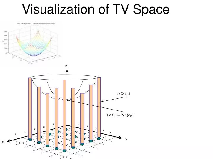
TV. TVX(x 15 ). TVX( )=TVX(x 33 ). 1. 1. 2. 2. 3. 3. 4. 4. 5. 5. Y. X. Visualization of TV Space. Proof that graph of TVX is a steep hyper-parabola centered at the mean, µ =( x X x i )/|X| Let f(c) = TVX(c) x X (x-c)o(x-c)

E N D
TV TVX(x15) TVX()=TVX(x33) 1 1 2 2 3 3 4 4 5 5 Y X Visualization of TV Space
Proof that graph of TVX is a steep hyper-parabola centered at the mean, µ=(xX xi)/|X| Let f(c) = TVX(c) xX (x-c)o(x-c) = xXi=1..n (xi - ci)2 = xX i=1..n (xi)2 - 2*x in X i=1..n xi*ci + xXi=1..n ci2 This is clearly parabolic in each dimension, ci (fixing all other dimensions) f/ck = xX -2(xk - ck) =0 iff xXxk = xXck = |X|ck iff ck = (xXxk)/|X| = µ We can say more about the shape of the hyper-parabolic graph of f. Since f/ck= xX -2(xk - ck) = -2xXxk + 2xXck = 2 xXck - 2|X|μk = 2|X|(ck -μk) we see that on each dimensional slice the parabola has the same shape, since the parabola in xy centered at (x0,y0) has the form y - y0 = a (x - x0)2 and a obviously = f(x0+1) -f(x0) we note y' =2a(x-x0), so in our case a=|X| a very large number (steep parabola) and x0 = µk Since the slope of the graph is |X|, if one wants, roughly, an -radius-contour (hyper-circular) centered at a, one needs to take the pre-image of the |X|-interval about TVX(a), f-1( TVX(a)- |X| , TVX(a)+ |X| )
a µ Proof that graph of IPX is a steep hyper-plane to µ = (xX xi)/|X| Inner Product functional: IPX(c) = xX xc = xX i=1..nxici = = i=1..n ci xXxi = i=1..n ci |X|µi= i=1..n ci |X|µi= |X| i=1..n ci µi= |X| cµ, so IPX(c) = |X| |µ| |c| cosθ where θ is the angle between c and µ. We can use any form of these equivalent formulas, depending upon which one sheds the most light on the issue we are concerned with. The blue one tell us what that the graph is extremely steep vertically (slight change in length of c causes a tremendous change in IPX(c) ) and that the contour(IPX,a,r) about a point, a, is a linear slice perpendicular to µ and also tells us how to choose the interval radius on the IPX axis so that the contour has radius, r. Red version guides to efficient preprocessing. The steepness of the graph is evident from f/ ck = |X|µk or the gradient, f = |X| |µ 1 1 2 2 3 3 4 4 5 5 x2 X1
Proof that graph of Xais a 45ohyper-plane nearly to µ = (xX xi)/|X| aDomainA1..DomainAn, projection onto a, Xa(x)=xa =i=1..nxi*ai is a functional whose graph is a hyperplane at a 45 angle with a. Contour(Xa,X,b,r) is a linear (n-1)-dimensional hyper-bar through b perpendicular to a. Xi(x) = xi is just Xei which also has planar graphs and have linear hyper-slice (n-1 dimensional) contours perpendicular to their coordinate basis vector, ei. Xa is just as easily calculated as TV (easier!), but which ones? All of them? That's impractical! One could process each Xi though. To classify all s in S, we could first cluster S based on some notion of closeness (isotropic clusters), then take the cluster means as representatives of the entire cluster, classify those cluster means individually (giving the same class assignment to all other points in that cluster, addressing the curse of cardinality of S), or we can classify each s in S individually. In either case we the classify s in S as follows: For unclassified sample (mean of cluster or just any sample), s, find a set of epsilon contours (from TVX, IPX, Xi's ) that reduce the candidate near neighbor set to a manageable size. Select the candidate near neighbors that are Euclidean close enough (or the closest k of them). Let those selected near nbrs vote with Gaussian Radial Basis (RDF) weighted votes. Done!
To prune halos with a small number of contours (fewer that the n+1 contours: {TV; Xi, i=1..n}, e.g., with 2 contours, use the Xa-µ-contour or use just a few Xi-contours corresponding to the largest coordinates of a-µ X1(a+ε X1(a-ε X2(a)+ε Xa-μ(a)+ε IPX(a)+ε Xa-μ(a)-ε X2(a)-ε IPX(a)-ε no halo, not too large no halo,but very large halos, but small a µ TVX(a)-ε TVX(a)+ε
c b a a ContourIPX(c,r) ContourTVX(a,r) 1 1 2 2 3 3 4 4 5 Γ 5 Xy(a) Contours of TVX, IPX, Xa, Xa-μ μ Y X ContourXy(a,r) 1 1 2 2 3 3 4 4 5 5 μ a Y X ContourXx(a,r) ContourXa-μ(a,r) 1 1 2 2 3 3 4 4 5 5 a-μ μ Y Γ X Note: ContourTVX(a,r) = Contour(TV,X,a,r), etc. ContourXb(a,r)
two (n-1)-D hypersurfaces (isobars) bounding ContourXa (a,r) ContourXy (a,r) outside surface of (n-1)D surface, ContourTVX(a,r) outside surface of ContourTVX(a,r) How about higher dimensions?
101 . . 1 100 . . 1 101 . . 1 001 . . 1 101 . . 1 111 . . 1 100 . . 1 101 . . 1 100 . . 1 101 . . 1 100 . . 1 101 . . 1 100 . . 1 101 . . 1 101 . . 1 100 . . 0 101 . . 0 101 . . 1 100 . . 1 0 1 2 3 8 9 11 12 13 14 15 20 21 22 23 28 29 30 31 leaf length Type0: pure0 leaves omitted. pure1s tagged in Purity Field. Purity Field (PF) Leaf Existence Array, LA 0 0 0 0 1 0 0 0 0 0 0 0 0 0 0 0 0 0 0 0 Leaf Existence Map, LM(size=NOPL) Leaf Map (LM) 0 1 1 1 1 0 0 0 0 1 1 0 1 1 1 1 1 0 0 0 0 1 1 1 1 0 0 0 0 1 1 1 1 0 1 2 3 4 5 6 7 8 9 10 11 12 13 14 15 16 17 18 19 20 21 22 23 24 25 26 27 28 29 30 31 1 0 0 . . 1 1 0 0 . . 1 1 0 1 . . 1 1 0 1 . . 1 1 0 0 . . 1 1 0 0 . . 1 1 0 1 . . 1 1 0 1 . . 1 1 0 1 . . 1 1 0 1 . . 1 0 0 1 . . 1 0 0 1 . . 1 1 0 1 . . 1 1 0 1 . . 1 1 0 0 . . 1 1 0 0 . . 1 1 0 0 . . 1 1 0 0 . . 1 1 0 1 . . 1 1 0 1 . . 1 1 0 1 . . 1 1 0 1 . . 1 1 0 0 . . 1 1 0 0 . . 1 1 0 1 . . 1 1 0 1 . . 1 1 0 1 . . 1 1 0 1 . . 1 1 0 0 . . 0 1 0 0 . . 0 1 0 1 . . 0 1 0 1 . . 0 1 0 1 . . 1 1 0 1 . . 1 1 0 0 . . 1 1 0 0 . . 1 0 0 0 0 0 0 0 0 0 0 0 0 0 0 0 0 0 0 0 0 0 1 0 0 0 0 0 0 0 0 0 0 Purity Map (PM) Ex.:dimension=1 fanout=2dimensoin=2 depth=5 NumberOfPotentialLeaves=NOPL=32=fanoutdepth Type-0 P-trees The upper inode levels are not productive. Indicate which leaves are either mixed or pure1 in a Leaf Existence Array (LA) with Purity Field (PF) or Leaf Existence Map (LM) and Purity Map (PM) Only the mixed leaves that get stored. Leaves are bit vectors, any or all of which could be compressed the same way (i.e., this 2-level structure can be nested to more levels). The LM is a "existential smoothing" of the Ptree (tells us precisely which leaves contain at least 1 1-bit). If we next enough, the LMs give us multiple smoothing levels. Needless to say, I prefer the LM/PM approach. The LM/PF may be clearer
Purity Field Type 0 means pure0 leaves omitted, pure1s switched on 0 0 0 0 1 0 0 0 0 0 0 0 0 0 0 0 0 0 0 0 0 1 2 3 8 9 11 12 13 14 15 20 21 22 23 28 29 30 31 Type1 means pure1 omitted, pure0s tagged in Purity Field. Purity Field (PF) Physical Structure: Leaf Exists Array or LA 1 0 0 0 1 0 0 0 0 0 0 1 0 0 0 0 0 1 0 0 0 0 1 1 10 0 1 2 3 8 9 12 13 14 15 16,17,18,19 20 21 22 23 24,25,26,27 28 29 30 31 4,5,6,7 11 1 0 0 . . 1 1 0 1 . . 1 1 0 0 . . 1 1 0 1 . . 1 1 0 1 . . 1 0 0 1 . . 1 1 0 1 . . 1 1 0 0 . . 1 1 0 0 . . 1 1 0 1 . . 1 1 0 1 . . 1 1 0 0 . . 1 1 0 1 . . 1 1 0 1 . . 1 1 0 0 . . 0 1 0 1 . . 0 1 0 1 . . 1 1 0 0 . . 1 Physical Structure: Leaf Exists Map or LM(size=NOPL=32) Leaf Map (LM) 1 1 1 1 1 0 0 0 0 1 1 0 1 1 1 1 1 0 0 0 0 1 1 1 1 0 0 0 0 1 1 1 1 0 1 2 3 4 5 6 7 8 9 10 11 12 13 14 15 16 17 18 19 20 21 22 23 24 25 26 27 28 29 30 31 1 0 0 . . 1 1 0 0 . . 1 1 0 1 . . 1 1 0 1 . . 1 1 0 0 . . 1 1 0 0 . . 1 1 0 1 . . 1 1 0 1 . . 1 1 0 1 . . 1 1 0 1 . . 1 0 0 1 . . 1 0 0 1 . . 1 1 0 1 . . 1 1 0 1 . . 1 1 0 0 . . 1 1 0 0 . . 1 1 0 0 . . 1 1 0 0 . . 1 1 0 1 . . 1 1 0 1 . . 1 1 0 1 . . 1 1 0 1 . . 1 1 0 0 . . 1 1 0 0 . . 1 1 0 1 . . 1 1 0 1 . . 1 1 0 1 . . 1 1 0 1 . . 1 1 0 0 . . 0 1 0 0 . . 0 1 0 1 . . 0 1 0 1 . . 0 1 0 1 . . 1 1 0 1 . . 1 1 0 0 . . 1 1 0 0 . . 1 0 0 0 0 1 1 1 1 0 0 0 0 0 0 0 0 0 0 0 0 0 1 0 0 0 0 0 0 0 0 0 0 Purity Map (PM) Physical Structure: Leaf Existence Array or LA Type-1 P-trees The Type-0 Ptree above, can be expressed as Type-1: Using either a Leaf Existence Array (LA) with Pure Field (PF) or a Leaf Existence Map (LM) and a Purity Map (PM)
How should Ptree be stored? impure leaves 0p1 101000101000011 leaf length 0p2 1p3 0p4 1p5 0p6 1 1 1 1 Leaf Map1 1 1 Leaf Map2 1 1 1 Leaf Map3 1 1 Leaf Map4 1 1 Leaf Map5 1 1 Leaf Map6 1 Pure Map1 1 Pure Map2 Pure Map3 1 Pure Map4 Pure Map5 1 1 Pure Map6 Type bit The tempting way to store these structures is to cluster by Ptree (horizontally across the rows of this cube above). But since those leaves almost never get ANDed with oneanother (except 1-time preprocessing) better to cluster by Leaf Offset or LM position ? ( vertically down this cube) since these are precisely the bit vectors that get ANDed together. If there is good compression (not too many mixed leaves per Ptree), then storing each Leaf Offset (vertical slice of the cube) on a page (or extent), would mean that only that page would need to be brought in when an actual AND is called for (and prefetching is straight forward). The collection of LMs and PMs could be stored separately on one extent, since they're processed separately (before) the leaves (or processed as smoothings).
011 1 . 1 011 . . 0 000 . . 0 111 . . 0 000 . . 0 010 . . 0 1 0 6 1 7 16 17 1 18 19 011 1 . 1 011 . . 0 111 . . 0 010 . . 0 6 1 7 16 17 1 18 19 100 . . 0 100 . . 1 111 . . 1 000 . . 1 111 . . 1 101 . . 1 000 . . 1 100 . . 1 101 . . 1 100 . . 0 P-tree operation: COMPLEMENT <-- COMPLEMENTing a P-tree --> Flip the Type Bit and complement the Leaves ( That's all!) If the structure is nested, complement a leaf by flipping its TypeBit and complementing its leaves (leaves of the leaves), etc.
101000000000011 101000101000011 101000111110011 101000101000000 111000000000011 111100101000011 000000000011011 0p1 0p2 1p3 0p4 000011000000001 000011000010101 1p5 0p6 1 1 1 1 0-Leaf Map1 1 1 0-Leaf Map2 1 1 1 1-Leaf Map3 1 1 0-Leaf Map4 1 1 1-Leaf Map5 1 1 0-Leaf Map6 1 0Pure Map1 1 0Pure Map2 2. pos=1, PM3(1)=0 so fetch & AND p1 101000101000011 p3 111100101000011 1Pure Map3 p6 000011000010101 res 000000000000001 1 0Pure Map4 1Pure Map5 1 1 0Pure Map6 P-tree operation: AND 0 1 2 3 4 5 6 7 8 9 positions Assumemixed leaves are clustered by Leaf Offset ( vertically down the cube), and the collection of LMs (and PMs) are stored separately on one additional extent. 1. AND all 0-LMs --> A 2. scan l-to-r across A for next 1 bit, if that position in any 1-PM=1, then GOTO 2 else fetch & AND nonpure leaves --> B; GOTO 2 3. A forms the LM of the result and the Bs are the nonpure leaves. E.g., p1 ^ p3 ^ p6 1. 1001100001^ 1000001001^ 1000010000= 1000000000 3. Result Ptree: 0-Leaf_Map: 1000000000 0-Pure_Map: 0000000000 impure leaves:000000000000001 root-count =1 Even better: ^{0LM} ^{1PM'} 0LM (result is always type0) Fetch & AND leaves corresp. to 1-bits in 0LM. Set Purity Map. In ASM, is there an operation, AND and COUNT? to count 1-bits as they are produced?
K 1 2 3 4 5 6 7 8 9 a b c d e f g h i j k l m n o p q r s t u v w x y z A B C D E F G H I J K L M N O P Q R S T U 5 6 1 3 0 0 0 0 0 0 0 0 0 0 0 0 0 0 0 0 0 0 0 0 0 0 0 0 0 1 1 1 1 1 1 1 0 0 0 0 0 0 0 0 0 0 0 0 0 0 0 0 0 0 0 0 0 0 0 0 7 1 2 0 0 0 0 0 0 0 0 0 0 0 0 0 0 0 0 0 0 0 0 0 0 0 0 1 0 1 1 1 1 0 1 0 0 1 1 1 0 1 0 1 0 1 0 0 1 1 1 1 1 1 1 1 1 1 1 2 3 1 1 0 0 1 1 0 0 1 1 0 0 1 1 0 0 1 1 0 1 0 1 0 1 0 1 0 1 1 1 1 1 1 1 1 1 0 0 1 1 1 1 1 1 1 1 1 0 0 1 0 1 0 0 1 0 1 0 3 4 1 0 0 1 0 1 0 1 0 1 0 1 0 1 0 1 0 1 1 1 0 0 1 1 0 0 0 1 0 1 0 1 0 0 0 1 0 1 0 0 0 0 0 0 0 0 1 0 1 0 0 0 0 1 1 0 0 1 22 2 3 0 0 0 0 0 0 0 0 0 0 0 0 0 0 0 0 0 0 0 0 0 0 0 0 0 1 1 1 1 1 0 0 1 1 11111111111111 1 0 0 0 0 0 0 0 2 1 2 2 0 0 0 0 0 0 0 0 0 0 0 0 0 0 0 0 1 1 1 1 1 1 1 1 1 1 1 1 1 1 1 0 1 1 1 1 1 1 1 1 1 1 1 0 0 0 0 0 1 1 1 1 1 1 1 1 3 4 2 1 0 0 0 0 0 0 0 0 1 1 1 1 1 1 1 1 0 0 0 0 1 1 1 1 1 1 1 1 1 1 1 0 1 1 1 1 1 1 1 0 0 0 0 1 1 1 1 1 0 1 1 1 1 0 0 0 3 5 2 0 0 0 0 0 1 1 1 1 0 0 0 0 1 1 1 1 0 0 1 1 0 0 1 1 1 0 0 0 1 1 1 1 1 1 1 1 1 0 0 1 1 0 0 1 1 1 1 1 1 1 0 0 0 1 1 0 3 3 13 00000000 00000000 00000000 01111111 00000000 00000000 00000000 12 00000000 00000000 00000000 10111101 00111010 10100111 11111111 11 00110011 00110011 01010101 01111111 11001111 11111001 01001010 10 01010101 01010101 11001100 01010100 01010000 00001010 00011001 13 0 0 0 1 0 0 0 0-p13 01111111 12 0 0 0 0 0 0 1 12 0 0 0 1 1 1 1 0-p12 10111101 00111010 10100111 11 1 1 1 1 1 1 1 1-p11 00110011 00110011 01010101 01111111 11001111 11111001 01001010 10 1 1 1 1 1 1 1 0-p10 01010101 01010101 11001100 01010100 01010000 00001010 00011001 22 1 1 0 1 0 1 0 22 1 1 0 0 0 0 0 0-p23 01111100 10000000 1-p22 11111110 11100000 1-p21 00001111 11111110 11111110 00011111 01111000 0-p20 00001111 00001111 00110011 10001111 11111001 10011111 11000110 23 0 0 0 0 1 1 0 23 0 0 0 1 1 1 1 20 1 1 1 1 1 1 1 23 00000000 00000000 00000000 01111100 11111111 11111111 10000000 22 00000000 00000000 11111111 11111110 11111111 11100000 11111111 21 00000000 11111111 00001111 11111110 11111110 00011111 01111000 20 00001111 00001111 00110011 10001111 11111001 10011111 11000110 21 1 0 1 1 1 1 1 21 1 0 0 0 0 0 0 LeafSize=8, NOPL=7 LeafOff=0; 11 10 20 001100110101010100001111 LeafOff=1; 11 10 20 001100110101010100001111 Leaf Maps (red are type-1) LeafOff=2; 11 10 21 2001010101110011000000111100110011 11 1 1 1 1 1 1 1 10 1 1 1 1 1 1 1 13 0 0 0 1 0 0 0 12 0 0 0 1 1 1 1 23 0 0 0 1 1 1 1 22 1 1 0 1 0 1 0 21 1 0 1 1 1 1 1 20 1 1 1 1 1 1 1 LeafOff=3; 13 12 11 1023 22 21 200111111110111101 011111110101010001111100111111101111111010001111 LeafOff=4; 12 11 10 21 20001110101100111101010000 1111111011111001 Purity Maps LeafOff=5; 12 11 10 22 21 20101001111111100100001010 111000000001111110011111 23 0 0 0 0 1 1 0 22 1 1 0 0 0 0 0 21 1 0 0 0 0 0 0 12 0 0 0 0 0 0 1 LeafOff=6; 11 10 23 21 20 010010100001100110000000 0111100011000110
P13^p12 13 0 0 0 1 0 0 0 12 0 0 0 1 1 1 1 0LM 0 0 0 1 0 0 0 P11^p10 ^{0LM} ^{1PM'} 0LM Fetch & AND lo=0,1,2,3,4,5,6 10 1 1 1 1 1 1 1 LM 1 1 1 1 1 1 1 ^{0LM}^{1PM'} 0LM lo=0; 11 10 00110011 0101010100010001 rc=2 lo=4; 11 10 11001111 0101000001000000 rc=1 Fetch & AND lo=3 lo3; 13 12 01111111 10111101 00111101 rc=5 lo=1; 11 10 00110011 0101010100010001 rc=2 lo=5; 11 1011111001 0000101000001000 rc=1 lo=2; 11 10 01010101 1100110001000100 rc=2 lo=6; 11 1001001010 00011001 00001000 rc=1 lo=3; 11 1001111111 0101010001010100 rc=3 Total rc=12 LeafMaps; (red=type1) lo0; 11 10 20 001100110101010100001111 11 1 1 1 1 1 1 1 10 1 1 1 1 1 1 1 13 0 0 0 1 0 0 0 12 0 0 0 1 1 1 1 23 0 0 0 1 1 1 1 22 1 1 0 1 0 1 0 21 1 0 1 1 1 1 1 20 1 1 1 1 1 1 1 lo1; 11 10 20 001100110101010100001111 lo2; 11 10 21 2001010101110011000000111100110011 lo3; 13 12 11 1023 22 21 200111111110111101011111110101010001111100111111101111111010001111 lo4; 12 11 10 21 200011101011001111010100001111111011111001 PureMaps; 23 0 0 0 0 1 1 0 22 1 1 0 0 0 0 0 21 1 0 0 0 0 0 0 12 0 0 0 0 0 0 1 lo5; 12 11 10 22 21 20101001111111100100001010111000000001111110011111 lo6; 11 10 23 21 20 0100101000011001100000000111100011000110
P22^p21 ^{0LM} ^{1PM'} 0LM Fetch & AND lo of 0LM 1-bit positions (i.e., 2,3,4,5,6) for P21, p22 (those that exits) 22' 0 0 1 1 1 1 1 21' 0 1 1 1 1 1 1 LM 0 0 1 1 1 1 1 00001111 rc=4 11111110 rc=7 11111110 rc=7 00000000 rc=0 01111000 rc=4 lo2; 21 00001111 lo3; 2211111110 21 11111110 lo4; 2111111110 lo5; 2211100000 21 00011111 lo6; 21 01111000 Total rc=22 LeafMaps; (red=type1) lo0; 11 10 20 001100110101010100001111 11 1 1 1 1 1 1 1 10 1 1 1 1 1 1 1 13 0 0 0 1 0 0 0 12 0 0 0 1 1 1 1 23 0 0 0 1 1 1 1 22 1 1 0 1 0 1 0 21 1 0 1 1 1 1 1 20 1 1 1 1 1 1 1 lo1; 11 10 20 001100110101010100001111 lo2; 11 10 21 2001010101110011000000111100110011 lo3; 13 12 11 1023 22 21 200111111110111101011111110101010001111100111111101111111010001111 lo4; 12 11 10 21 200011101011001111010100001111111011111001 PureMaps; 23 0 0 0 0 1 1 0 22 1 1 0 0 0 0 0 21 1 0 0 0 0 0 0 12 0 0 0 0 0 0 1 lo5; 12 11 10 22 21 20101001111111100100001010111000000001111110011111 lo6; 11 10 23 21 20 0100101000011001100000000111100011000110
22' 0 0 1 1 1 1 1 21' 0 1 1 1 1 1 1 13 0 0 0 1 0 0 0 12 0 0 0 1 1 1 1 P22^p21^p13^p12 ^{0LM} ^{1PM'} 0LM Fetch & AND lo of 0LM 1-bit positions (i.e., lo3) for 21, 22 13, 12 (those that exits) LM 0 0 0 1 0 0 0 lo3; 13 12 22 21 01111111 10111101 11111110 11111110 00111100 rc=4 LeafMaps; (red=type1) lo0; 11 10 20 001100110101010100001111 11 1 1 1 1 1 1 1 10 1 1 1 1 1 1 1 13 0 0 0 1 0 0 0 12 0 0 0 1 1 1 1 23 0 0 0 1 1 1 1 22 1 1 0 1 0 1 0 21 1 0 1 1 1 1 1 20 1 1 1 1 1 1 1 lo1; 11 10 20 001100110101010100001111 lo2; 11 10 21 2001010101110011000000111100110011 lo3; 13 12 11 1023 22 21 200111111110111101011111110101010001111100111111101111111010001111 lo4; 12 11 10 21 200011101011001111010100001111111011111001 PureMaps; 23 0 0 0 0 1 1 0 22 1 1 0 0 0 0 0 21 1 0 0 0 0 0 0 12 0 0 0 0 0 0 1 lo5; 12 11 10 22 21 20101001111111100100001010111000000001111110011111 lo6; 11 10 23 21 20 0100101000011001100000000111100011000110
P22^p21 ^{0LM} ^{1PM'} 0LM Fetch & AND lo of 0LM 1-bit positions (i.e., 2,3,4,5,6) for P21, p22 (those that exits) 22' 0 0 1 1 1 1 1 21' 0 1 1 1 1 1 1 LM 0 0 1 1 1 1 1 00001111 rc=4 11111110 rc=7 11111110 rc=7 00000000 rc=0 01111000 rc=4 lo2; 21 00001111 lo3; 2211111110 21 11111110 lo4; 2111111110 lo5; 2211100000 21 00011111 lo6; 21 01111000 Total rc=22 LeafMaps; (red=type1) lo0; 11 10 20 001100110101010100001111 11 1 1 1 1 1 1 1 10 1 1 1 1 1 1 1 13 0 0 0 1 0 0 0 12 0 0 0 1 1 1 1 23 0 0 0 1 1 1 1 22 1 1 0 1 0 1 0 21 1 0 1 1 1 1 1 20 1 1 1 1 1 1 1 lo1; 11 10 20 001100110101010100001111 lo2; 11 10 21 2001010101110011000000111100110011 lo3; 13 12 11 1023 22 21 200111111110111101011111110101010001111100111111101111111010001111 lo4; 12 11 10 21 200011101011001111010100001111111011111001 PureMaps; 23 0 0 0 0 1 1 0 22 1 1 0 0 0 0 0 21 1 0 0 0 0 0 0 12 0 0 0 0 0 0 1 lo5; 12 11 10 22 21 20101001111111100100001010111000000001111110011111 lo6; 11 10 23 21 20 0100101000011001100000000111100011000110
Vertical Data Assistant (VDA)is a windows (or windows CE) application that can data mine massive datasets efficiently? (note that the a separate application can be built to convert an store properly. I am changing my thinking a bit on DataMIME and the whole idea of competing in the "big iron" community with a data mining system. There is no way to win there (too many players with too much money - Google, Microsoft, all the Bioinformatics and Drug development companies....). It occurred to me, as I was revising Masum's slides, that other than the size of the datasets, our methods and modules are getting surprisingly simple and compact. Developing DataMIME on big hardware may be a mistake, if no one uses it! Maybe it is wrong-headed? Maybe the killer app is a completely portable, tiny client system (on a desktop/laptop/PDA) that can do scalable data mining for "anyone, anytime, anywhere" provided their data is capture into a consistent universally format. If this would work, it could eventually be scaled up to supercomputers and as a Grid App, but first, let's do a tiny version (tiny in terms of system requirements, but not in terms of DM power). DataSURG software development (e.g., SMILEY, DataMIME) weren't too successful. The one software system has been used is TM-Lab, a small app on small PCs and requiring data be in a simple format (BSQ). I now favor a Windows and Windows CE Utility Suite approach. Each Utility does one thing we and can be invoked in a GUI drag and drop mode. (e.g., An AND operation pulls the specified Ptrees from the specified folder and returns either just the rootcount or drops the resulting "derived Ptree" back in the folder and returns its name. Each platform (PDA to supercomputer) will get an appropriate subset of the suite.
Body Area Network (BAN) and Network is the Computer (NITC) technologies may eventually converge to produce the next "sea change" technology. Imagine nano-computers, massive storage (e.g., 4G thumb drives), a wireless networks and applications such as real-time health monitors (blood_emzynes/body_temperature/blood_sugar/coronary_flow...); PDA apps (schedulers/reminders/auto_thought_recorders, DNA/FingerPrint/FaceGeo/IrisScan realtime name_recall/restraining_order_enforcement/homeland_security); Environmental sensors (eyes_in_back_of_head/sense_nearby_explosives/viruses_sensing...). All that data will have to be data mined for exceptions. Exception mining (i.e., classification into 2 classes, exceptional_situation or normal_situation) is what DataSURG does better than anyone in the world (add "ego monitoring" to VDA apps ;-) Our approach can be implemented on tiny processing platforms. Of course the datasets are large, so they must be broken up and compressed and store in an extremely simple and universal (no variations!) format. So simple that Windows CE can handle them and so that Joe Public can understand them. After all, simplicity and consistency made the Relational Model successful!
x y z A B C D E N F G H I J K L M 1111 1110 1101 1100 1011 1010 1001 1000 t u r s q n o l m j k h i • p O P Q R S T U V v 0111 0110 0101 0100 0011 0010 0001 0000 d e f g 9 a b c 5 6 7 8 1 2 3 4 w 0000 0001 0010 0011 0100 0101 0110 0111 1000 1001 1010 1011 1100 1101 1110 1111 K 1 2 3 4 5 6 7 8 9 a b c d e f g h i j k l m n o p q r s t u v w x y z A B C D E F G H I J K L M N O P Q R S T U V 5 7 1 3 0 0 0 0 0 0 0 0 0 0 0 0 0 0 0 0 0 0 0 0 0 0 0 0 0 1 1 1 1 1 1 1 0 0 0 0 0 0 0 0 0 0 0 0 0 0 0 0 0 0 0 0 0 0 0 0 0 7 1 2 0 0 0 0 0 0 0 0 0 0 0 0 0 0 0 0 0 0 0 0 0 0 0 0 1 0 1 1 1 1 0 1 0 0 1 1 1 0 1 0 1 0 1 0 0 1 1 1 1 1 1 1 1 1 1 1 1 2 4 1 1 0 0 1 1 0 0 1 1 0 0 1 1 0 0 1 1 0 1 0 1 0 1 0 1 0 1 1 1 1 1 1 1 1 1 0 0 1 1 1 1 1 1 1 1 1 0 0 1 0 1 0 0 1 0 1 0 1 3 5 1 0 0 1 0 1 0 1 0 1 0 1 0 1 0 1 0 1 1 1 0 0 1 1 0 0 0 1 0 1 0 1 0 0 0 1 0 1 0 0 0 0 0 0 0 0 1 0 1 0 0 0 0 1 1 0 0 1 1 23 2 3 0 0 0 0 0 0 0 0 0 0 0 0 0 0 0 0 0 0 0 0 0 0 0 0 0 1 1 1 1 1 0 0 1 1 11111111111111 1 0 0 0 0 0 0 0 0 2 2 2 2 0 0 0 0 0 0 0 0 0 0 0 0 0 0 0 0 1 1 1 1 1 1 1 1 1 1 1 1 1 1 1 0 1 1 1 1 1 1 1 1 1 1 1 0 0 0 0 0 1 1 1 1 1 1 1 1 1 3 5 2 1 0 0 0 0 0 0 0 0 1 1 1 1 1 1 1 1 0 0 0 0 1 1 1 1 1 1 1 1 1 1 1 0 1 1 1 1 1 1 1 0 0 0 0 1 1 1 1 1 0 1 1 1 1 0 0 0 0 3 5 2 0 0 0 0 0 1 1 1 1 0 0 0 0 1 1 1 1 0 0 1 1 0 0 1 1 1 0 0 0 1 1 1 1 1 1 1 1 1 0 0 1 1 0 0 1 1 1 1 1 1 1 0 0 0 1 1 0 0 3 3 µi = (xX xi) / |X| =(1/57)x k 2kxi, (1/57)k 2kxxi,k =(1/57)k 2krcPi,k for i=1 =(1/57)*(7*23 +24*22+35*21+23*20) =4.3 µ for i=2 =(1/57)*(22*23 +35*22+35*21+33*20) =7.35 Created a bit map for each {ring(f,Y,k)}k=1..K , of each Y={x}, one would have all reverse-kNN information and much more! ring(f,Y,k)s give up distance information, so {ring(f,Y,(kr, (k+1)r])}k=0..R holds more info, but makes it more difficult to computer reverse-kNN sets (though more useful sets can easily be calculated to do a better job of whatever reverse-kNN sets were to be used for anyway).
rx1,1,k x y z A B C D E N F G H I J K L M 1111 1110 1101 1100 1011 1010 1001 1000 t u r s q n o l m j k h i • p O P Q R S T U V v 0111 0110 0101 0100 0011 0010 0001 0000 d e f g 9 a b c 5 6 7 8 1 2 3 4 w 0000 0001 0010 0011 0100 0101 0110 0111 1000 1001 1010 1011 1100 1101 1110 1111 3 0 0 1 0 1 0 1 0 1 1 0 0 1 0 1 0 1 1 1 0 0 1 1 0 0 0 0 0 0 0 0 0 0 0 1 0 0 0 0 0 0 0 0 0 0 1 0 0 0 0 0 0 0 0 0 0 0 0 1 4 3 1 1 0 0 0 1 0 0 0 1 0 0 0 1 0 0 0 0 0 1 0 0 0 1 0 1 0 0 0 0 0 0 0 0 0 1 0 0 0 0 0 0 0 0 0 0 1 0 0 1 0 1 0 0 1 0 0 0 1 2 3 2 0 0 0 0 0 0 0 0 0 0 0 0 0 0 0 0 0 0 0 0 0 0 0 0 0 0 0 0 0 0 0 0 0 0 0 1 1 0 1 0 1 0 1 0 0 0 1 1 0 1 0 1 0 0 1 1 0 1 1 K 1 2 3 4 5 6 7 8 9 a b c d e f g h i j k l m n o p q r s t u v w x y z A B C D E F G H I J K L M N O P Q R S T U V 5 7 1 3 0 0 0 0 0 0 0 0 0 0 0 0 0 0 0 0 0 0 0 0 0 0 0 0 0 1 1 1 1 1 1 1 0 0 0 0 0 0 0 0 0 0 0 0 0 0 0 0 0 0 0 0 0 0 0 0 0 7 1 2 0 0 0 0 0 0 0 0 0 0 0 0 0 0 0 0 0 0 0 0 0 0 0 0 1 0 1 1 1 1 0 1 0 0 1 1 1 0 1 0 1 0 1 0 0 1 1 1 1 1 1 1 1 1 1 1 1 2 4 1 1 0 0 1 1 0 0 1 1 0 0 1 1 0 0 1 1 0 1 0 1 0 1 0 1 0 1 1 1 1 1 1 1 1 1 0 0 1 1 1 1 1 1 1 1 1 0 0 1 0 1 0 0 1 0 1 0 1 3 5 1 0 0 1 0 1 0 1 0 1 0 1 0 1 0 1 0 1 1 1 0 0 1 1 0 0 0 1 0 1 0 1 0 0 0 1 0 1 0 0 0 0 0 0 0 0 1 0 1 0 0 0 0 1 1 0 0 1 1 23 2 3 0 0 0 0 0 0 0 0 0 0 0 0 0 0 0 0 0 0 0 0 0 0 0 0 0 1 1 1 1 1 0 0 1 1 11111111111111 1 0 0 0 0 0 0 0 0 2 2 2 2 0 0 0 0 0 0 0 0 0 0 0 0 0 0 0 0 1 1 1 1 1 1 1 1 1 1 1 1 1 1 1 0 1 1 1 1 1 1 1 1 1 1 1 0 0 0 0 0 1 1 1 1 1 1 1 1 1 3 5 2 1 0 0 0 0 0 0 0 0 1 1 1 1 1 1 1 1 0 0 0 0 1 1 1 1 1 1 1 1 1 1 1 0 1 1 1 1 1 1 1 0 0 0 0 1 1 1 1 1 0 1 1 1 1 0 0 0 0 3 5 2 0 0 0 0 0 1 1 1 1 0 0 0 0 1 1 1 1 0 0 1 1 0 0 1 1 1 0 0 0 1 1 1 1 1 1 1 1 1 0 0 1 1 0 0 1 1 1 1 1 1 1 0 0 0 1 1 0 0 3 3 1 0 0 1 0 0 0 1 0 0 0 1 0 0 0 1 0 0 1 0 0 0 1 0 0 0 0 0 0 0 0 0 0 0 0 0 0 0 0 0 0 0 0 0 0 0 0 0 0 0 0 0 0 0 0 0 0 0 0 6 1 1 0 0 1 0 0 0 1 0 0 0 1 0 0 0 1 0 0 0 0 1 0 0 0 1 0 0 0 0 0 0 0 0 1 0 0 0 0 1 0 1 0 1 0 1 0 0 0 0 0 0 0 0 0 0 0 0 0 1 1 1 2 0 0 0 1 0 0 0 1 0 0 0 1 0 0 0 1 0 1 0 0 0 1 0 0 1 0 0 0 0 0 0 0 0 1 1 0 0 0 0 0 0 0 0 0 1 1 0 0 1 0 1 0 0 1 0 0 0 1 4 2 0 1 0 1 0 1 0 1 0 1 0 1 0 1 0 1 0 0 0 1 1 0 0 1 1 0 0 0 0 0 0 0 0 1 0 0 0 0 1 0 1 0 1 0 1 0 0 0 0 0 0 0 0 0 0 0 0 0 1 7 2 1 0 0 0 1 0 0 0 1 0 0 0 1 0 0 0 1 0 1 0 0 0 1 0 0 0 0 0 0 0 0 0 0 0 1 0 0 0 0 0 0 0 0 0 0 1 0 0 0 0 0 0 0 0 0 0 0 0 8 2 2 0 0 0 0 0 0 0 0 0 0 0 0 0 0 0 0 0 0 0 0 0 0 0 0 1 0 0 0 0 0 0 0 0 0 1 1 0 0 0 0 0 0 0 0 0 1 1 0 1 0 1 1 0 1 0 1 0 1 0 µ We note that the ring(a,d*(k-1),d*k) tell an even greater story but they may have higher cost? ra,0=skin(a,1) ra,k=ring(a,2k-1,2k) ring(a,d*2k-1,d*2k ) k=0... tell a great story on neighbors. (here, d=1) rf,a,k=ring(f,f-1a,2k-1,2k)
x y z A B C D E N F G H I J K L M 1111 1110 1101 1100 1011 1010 1001 1000 t u r s q n o l m j k h i • p O P Q R S T U V v 0111 0110 0101 0100 0011 0010 0001 0000 d e f g 9 a b c 5 6 7 8 1 2 3 4 w 0000 0001 0010 0011 0100 0101 0110 0111 1000 1001 1010 1011 1100 1101 1110 1111 U 0 0 0 0 0 0 0 0 0 0 0 0 0 0 0 0 0 0 0 0 0 0 0 0 0 1 0 0 0 0 0 0 0 0 0 1 0 1 0 1 0 1 0 1 0 0 1 0 1 1 1 1 0 0 1 1 0 0 1 3 U 1 0 0 0 1 0 0 0 1 0 0 0 1 0 0 0 1 0 1 0 0 0 1 0 0 0 0 0 0 0 0 0 0 0 1 0 0 0 0 0 0 0 0 0 0 1 0 0 0 0 0 0 0 1 0 0 0 1 1 0 U 2 0 0 0 0 0 0 0 0 0 0 0 0 0 0 0 0 0 0 0 0 0 0 0 0 0 0 0 0 0 0 0 0 0 0 0 1 1 0 1 0 1 0 1 0 0 0 1 1 0 1 0 1 0 0 1 1 0 1 1 K 1 2 3 4 5 6 7 8 9 a b c d e f g h i j k l m n o p q r s t u v w x y z A B C D E F G H I J K L M N O P Q R S T U V 5 7 4 0 0 0 1 0 0 0 1 0 0 0 1 0 0 0 1 0 0 0 0 1 0 0 0 1 1 0 0 0 0 0 0 0 1 0 1 0 0 1 0 1 0 1 0 1 0 1 0 0 1 0 1 0 0 1 0 0 0 1 7 4 1 0 1 0 0 0 1 0 0 0 1 0 0 0 1 0 0 1 0 0 0 1 0 0 0 0 0 0 0 0 0 0 0 0 0 0 1 0 0 0 0 0 0 0 0 0 0 1 0 0 0 0 1 0 0 0 1 0 1 0 4 2 1 0 0 0 1 0 0 0 1 0 0 0 1 0 0 0 0 0 1 0 0 0 1 0 0 0 0 0 0 0 0 0 0 0 0 0 1 0 1 0 1 0 1 0 0 0 0 1 0 1 0 0 1 0 1 0 1 1 5 S 0 0 0 0 1 0 0 0 1 0 0 0 1 0 0 0 1 0 1 0 0 0 1 0 0 0 0 0 0 0 0 0 0 0 1 0 1 0 0 0 0 0 0 0 0 1 0 1 0 0 0 0 1 0 0 0 1 0 1 2 S 1 0 0 1 0 0 0 1 0 0 0 1 0 0 0 1 0 0 0 0 1 0 0 0 1 0 0 0 0 0 0 0 0 1 0 0 0 1 1 1 1 1 1 1 1 0 0 0 1 0 1 0 0 0 0 1 0 0 1 8 S 2 1 1 0 0 1 1 0 0 1 1 0 0 1 1 0 0 1 0 1 0 1 0 1 0 0 0 0 0 0 0 0 0 0 0 0 0 0 0 0 0 0 0 0 0 0 0 0 0 0 0 0 0 1 0 0 0 1 1 4 µ
x y z A B C D E N F G H I J K L M 1111 1110 1101 1100 1011 1010 1001 1000 t u r s q n o l m j k h i • p O P Q R S T U V v 0111 0110 0101 0100 0011 0010 0001 0000 d e f g 9 a b c 5 6 7 8 1 2 3 4 w 0000 0001 0010 0011 0100 0101 0110 0111 1000 1001 1010 1011 1100 1101 1110 1111 v 0 0 0 0 0 0 0 0 0 0 0 0 0 0 0 0 0 0 0 0 0 0 0 0 0 0 1 0 0 0 0 0 0 0 0 0 0 0 0 0 0 0 0 0 0 0 0 0 0 0 0 0 0 0 0 0 0 0 1 v 1 0 0 0 0 0 0 0 0 0 0 0 0 0 0 0 0 0 0 0 0 0 0 0 0 0 0 0 0 0 0 0 0 0 0 0 0 0 0 0 0 0 0 0 0 0 0 0 0 0 0 0 0 0 0 0 0 0 0 v 2 0 0 0 0 0 0 0 0 0 0 0 0 0 0 0 0 0 0 0 0 0 0 0 0 0 0 1 0 1 0 0 1 0 0 0 0 1 0 1 0 1 0 1 0 0 0 0 1 0 1 0 0 1 0 1 0 1 1 2 K 1 2 3 4 5 6 7 8 9 a b c d e f g h i j k l m n o p q r s t u v w x y z A B C D E F G H I J K L M N O P Q R S T U V 5 7 T 0 0 0 0 0 0 0 0 0 0 0 0 0 0 0 0 0 0 0 0 0 0 0 0 0 0 0 0 0 0 0 0 0 0 0 0 1 0 0 0 0 0 0 0 0 0 0 1 0 0 0 0 1 1 0 0 1 1 6 T 1 0 0 0 0 0 0 0 0 0 0 0 0 0 0 0 0 0 0 0 0 0 0 0 0 1 0 0 0 0 0 0 0 0 0 1 0 0 0 0 0 0 0 0 0 0 1 0 0 1 0 1 0 0 1 0 0 0 6 T 2 0 0 1 1 0 0 1 1 0 0 1 1 0 0 1 1 0 1 0 1 0 1 0 1 0 0 0 0 0 0 1 0 1 1 0 0 0 1 0 1 0 1 0 1 1 0 0 0 0 0 0 0 0 0 0 0 0 2 0 V 0 0 0 0 0 0 0 0 0 0 0 0 0 0 0 0 0 0 0 0 0 0 0 0 0 0 0 0 0 0 0 0 0 0 0 0 0 1 0 1 0 1 0 1 0 0 0 0 1 0 1 0 0 0 0 1 0 0 7 V 1 0 0 0 0 0 0 0 0 0 0 0 0 0 0 0 0 0 0 0 0 0 0 0 0 0 0 0 0 0 0 0 0 0 0 0 1 0 0 0 0 0 0 0 0 0 0 1 0 0 0 0 1 0 0 0 1 0 4 V 2 0 0 0 1 0 0 0 1 0 0 0 1 0 0 0 1 0 1 0 0 0 1 0 0 1 1 0 0 0 0 1 0 0 1 1 0 0 0 0 0 0 0 0 0 1 1 0 0 1 0 1 0 0 1 0 0 0 1 6 µ
x y z A B C D E N F G H I J K L M 1111 1110 1101 1100 1011 1010 1001 1000 t u r s q n o l m j k h i • p O P Q R S T U V v 0111 0110 0101 0100 0011 0010 0001 0000 d e f g 9 a b c 5 6 7 8 1 2 3 4 w 0000 0001 0010 0011 0100 0101 0110 0111 1000 1001 1010 1011 1100 1101 1110 1111 s 0 0 0 0 0 0 0 0 0 0 0 0 0 0 0 0 0 0 0 0 0 0 0 0 0 0 0 1 0 1 0 0 1 0 0 0 0 0 0 0 0 0 0 0 0 0 0 0 0 0 0 0 0 0 0 0 0 0 3 s 1 0 0 0 0 0 0 0 0 0 0 0 0 0 0 0 0 0 0 0 0 0 0 0 0 0 0 0 0 0 0 0 0 0 0 0 0 0 0 0 0 0 0 0 0 0 0 0 0 0 0 0 0 0 0 0 0 0 0 s 2 0 0 0 0 0 0 0 0 0 0 0 0 0 0 0 0 0 0 0 0 0 0 0 0 0 1 0 0 0 0 0 0 0 0 0 0 0 0 0 0 0 0 0 0 0 0 0 0 0 0 0 0 0 0 0 0 0 1 K 1 2 3 4 5 6 7 8 9 a b c d e f g h i j k l m n o p q r s t u v w x y z A B C D E F G H I J K L M N O P Q R S T U V 5 7 q 0 0 0 0 0 0 0 0 0 0 0 0 0 0 0 0 0 0 0 0 0 0 0 0 0 0 0 0 0 0 0 1 0 0 0 0 0 0 0 0 0 0 0 0 0 0 0 0 0 0 0 0 0 0 0 0 0 0 1 q 1 0 0 0 0 0 0 0 0 0 0 0 0 0 0 0 0 0 0 0 0 0 0 0 0 0 0 0 0 0 0 0 0 0 0 0 0 0 0 0 0 0 0 0 0 0 0 0 0 0 0 0 0 0 0 0 0 0 0 q 2 0 0 0 0 0 0 0 0 0 0 0 0 0 0 0 0 0 0 0 0 0 0 0 0 0 0 1 1 1 1 0 1 0 0 0 0 0 0 0 0 0 0 0 0 0 0 0 0 0 0 0 0 1 0 0 0 1 7 w 0 0 0 0 0 0 0 0 0 0 0 0 0 0 0 0 0 0 0 0 0 0 0 0 0 0 0 0 1 0 1 0 0 0 0 0 0 0 0 0 0 0 0 0 0 0 0 0 0 0 0 0 0 0 0 0 0 0 2 w 1 0 0 0 0 0 0 0 0 0 0 0 0 0 0 0 0 0 0 0 0 0 0 0 0 0 0 0 0 0 0 0 0 0 0 0 0 0 0 0 0 0 0 0 0 0 0 0 0 0 0 0 0 0 0 0 0 0 0 w 2 0 0 0 0 0 0 0 0 0 0 0 0 0 0 0 0 0 0 0 0 0 0 0 0 0 1 0 0 0 0 1 0 0 0 0 0 0 0 0 0 0 0 0 0 0 0 0 0 0 0 0 0 0 0 0 0 0 2
x y z A B C D E N F G H I J K L M 1111 1110 1101 1100 1011 1010 1001 1000 t u r s q n o l m j k h i • p O P Q R S T U V v 0111 0110 0101 0100 0011 0010 0001 0000 d e f g 9 a b c 5 6 7 8 1 2 3 4 w 0000 0001 0010 0011 0100 0101 0110 0111 1000 1001 1010 1011 1100 1101 1110 1111 9 0 0 0 0 0 1 1 1 1 0 0 0 0 1 1 1 1 0 0 0 0 0 0 0 0 0 0 0 0 0 0 0 1 0 0 0 0 0 0 0 0 0 0 0 0 0 0 0 0 0 0 0 0 0 0 0 0 0 9 9 1 1 1 1 1 0 0 0 0 0 0 0 0 0 0 0 0 1 1 0 0 0 0 0 0 0 0 0 0 0 0 0 0 0 0 0 0 0 0 0 0 0 0 0 0 0 0 0 0 0 0 0 0 0 0 0 1 1 8 9 2 0 0 0 0 0 0 0 0 0 0 0 0 0 0 0 0 0 0 1 1 1 1 0 0 0 0 0 0 0 0 0 0 0 0 0 0 0 0 0 0 0 0 0 0 0 0 0 0 0 0 1 1 1 1 1 0 0 9 K 1 2 3 4 5 6 7 8 9 a b c d e f g h i j k l m n o p q r s t u v w x y z A B C D E F G H I J K L M N O P Q R S T U V 5 7 1 0 0 0 0 0 1 1 1 1 0 0 0 0 0 0 0 0 0 0 0 0 0 0 0 0 0 0 0 0 0 0 0 1 0 0 0 0 0 0 0 0 0 0 0 0 0 0 0 0 0 0 0 0 0 0 0 0 0 5 1 1 0 0 0 0 0 0 0 0 1 1 1 1 0 0 0 0 0 0 0 0 0 0 0 0 0 0 0 0 0 0 0 0 0 0 0 0 0 0 0 0 0 0 0 0 0 0 0 0 0 0 0 0 0 0 0 0 0 4 1 2 0 0 0 0 0 0 0 0 0 0 0 0 1 1 1 1 1 1 0 0 0 0 0 0 0 0 0 0 0 0 0 0 0 0 0 0 0 0 0 0 0 0 0 0 0 0 0 0 0 0 0 0 0 0 0 1 1 8 5 0 1 1 1 1 0 0 0 0 1 1 1 1 0 0 0 0 0 0 0 0 0 0 0 0 0 0 0 0 0 0 0 0 0 0 0 0 0 0 0 0 0 0 0 0 0 0 0 0 0 0 0 0 0 0 0 0 0 8 5 1 0 0 0 0 0 0 0 0 0 0 0 0 1 1 1 1 0 0 0 0 0 0 0 0 0 0 0 0 0 0 0 0 0 0 0 0 0 0 0 0 0 0 0 0 0 0 0 0 0 0 0 0 0 0 0 0 0 4 5 2 0 0 0 0 0 0 0 0 0 0 0 0 0 0 0 0 1 1 1 1 0 0 0 0 0 0 0 0 0 0 0 0 0 0 0 0 0 0 0 0 0 0 0 0 0 0 0 0 0 0 0 0 0 1 1 1 1 8
x y z A B C D E N F G H I J K L M 1111 1110 1101 1100 1011 1010 1001 1000 t u r s q n o l m j k h i • p O P Q R S T U V v 0111 0110 0101 0100 0011 0010 0001 0000 d e f g 9 a b c 5 6 7 8 1 2 3 4 w 0000 0001 0010 0011 0100 0101 0110 0111 1000 1001 1010 1011 1100 1101 1110 1111 j 0 0 0 0 0 0 0 0 0 0 0 0 0 0 0 0 0 1 1 0 0 1 1 0 0 0 0 0 0 0 0 0 0 0 0 0 0 0 0 0 0 00 0 0 0 0 0 0 0 0 1 1 1 0 0 1 1 9 j 1 0 0 0 0 0 0 0 0 0 0 0 0 1 1 1 1 0 0 0 0 0 0 1 1 1 0 0 0 0 0 1 0 0 0 0 0 0 0 0 0 0 0 0 0 0 0 0 0 0 1 0 0 0 0 0 0 0 9 j 2 0 0 0 0 1 1 1 1 1 1 1 1 0 0 0 0 0 0 0 0 0 0 0 0 0 0 0 0 0 0 0 1 0 0 0 0 0 0 0 0 0 0 0 0 0 0 0 0 0 0 0 0 0 0 0 0 0 9 K 1 2 3 4 5 6 7 8 9 a b c d e f g h i j k l m n o p q r s t u v w x y z A B C D E F G H I J K L M N O P Q R S T U V 5 7 d 0 0 0 0 0 0 0 0 0 1 1 1 1 0 0 0 0 1 1 0 0 0 0 0 0 0 0 0 0 0 0 0 0 0 0 0 0 0 0 0 0 0 0 0 0 0 0 0 0 0 0 0 0 0 0 0 1 1 8 d 1 0 0 0 0 1 1 1 1 0 0 0 0 0 0 0 0 0 0 1 1 0 0 0 0 0 0 0 0 0 0 0 1 0 0 0 0 0 0 0 0 0 0 0 0 0 0 0 0 0 0 0 0 0 1 1 0 0 9 d 2 1 1 1 1 0 0 0 0 0 0 0 0 0 0 0 0 0 0 0 0 1 1 1 1 1 0 0 0 0 0 1 0 0 0 0 0 0 0 0 0 0 0 0 0 0 0 0 0 0 1 1 1 1 0 0 0 0 1 4 h 0 0 0 0 0 0 0 0 0 0 0 0 0 1 1 1 1 0 0 1 1 0 0 0 0 0 0 0 0 0 0 0 0 0 0 0 0 0 0 0 0 0 0 0 0 0 0 0 0 0 0 0 0 0 1 1 0 0 8 h 1 0 0 0 0 0 0 0 0 1 1 1 1 0 0 0 0 0 0 0 0 1 1 0 0 0 0 0 0 0 0 0 0 0 0 0 0 0 0 0 0 0 0 0 0 0 0 0 0 0 0 1 1 1 0 0 0 0 9 h 2 1 1 1 1 1 1 1 1 0 0 0 0 0 0 0 0 0 0 0 0 0 0 1 1 1 0 0 0 0 0 1 1 0 0 0 0 0 0 0 0 0 0 0 0 0 0 0 0 0 1 0 0 0 0 0 0 0 1 4
x y z A B C D E N F G H I J K L M 1111 1110 1101 1100 1011 1010 1001 1000 t u r s q n o l m j k h i • p O P Q R S T U V v 0111 0110 0101 0100 0011 0010 0001 0000 d e f g 9 a b c 5 6 7 8 1 2 3 4 w 0000 0001 0010 0011 0100 0101 0110 0111 1000 1001 1010 1011 1100 1101 1110 1111 K 1 2 3 4 5 6 7 8 9 a b c d e f g h i j k l m n o p q r s t u v w x y z A B C D E F G H I J K L M N O P Q R S T U V 5 7 l 0 0 0 0 0 0 0 0 0 0 0 0 0 0 0 0 0 0 0 1 1 0 0 1 1 1 0 0 0 0 0 1 0 0 0 0 0 0 0 0 0 0 0 0 0 0 0 0 0 0 1 0 0 0 1 1 0 0 9 l 1 0 0 0 0 0 0 0 0 0 0 0 0 0 0 0 0 1 1 0 0 0 0 0 0 0 0 0 0 0 0 0 0 0 0 0 0 0 0 0 0 0 0 0 0 0 0 0 0 0 0 0 0 0 0 0 1 1 4 l 2 0 0 0 0 0 0 0 0 1 1 1 1 1 1 1 1 0 0 0 0 0 0 0 0 0 0 0 0 0 0 0 0 0 0 0 0 0 0 0 0 0 0 0 0 0 0 0 0 0 0 0 0 0 0 0 0 0 8 n 0 0 0 0 0 0 0 0 0 0 0 0 0 0 0 0 0 0 0 0 0 1 1 0 0 0 0 0 0 0 0 0 0 0 0 0 0 0 0 0 0 0 0 0 0 0 0 0 0 0 0 1 1 1 0 0 0 0 5 n 1 0 0 0 0 0 0 0 0 0 0 0 0 0 0 0 0 0 0 1 1 0 0 0 0 0 0 0 0 0 0 0 0 0 0 0 0 0 0 0 0 0 0 0 0 0 0 0 0 0 0 0 0 0 1 1 0 0 4 n 2 0 0 0 0 0 0 0 0 0 0 0 0 1 1 1 1 1 1 0 0 0 0 0 0 0 0 0 0 0 0 0 0 0 0 0 0 0 0 0 0 0 0 0 1 1 1 1 1 0 0 0 0 0 0 0 1 1 1 3
x y z A B C D E N F G H I J K L M 1111 1110 1101 1100 1011 1010 1001 1000 t u r s q n o l m j k h i • p O P Q R S T U V v 0111 0110 0101 0100 0011 0010 0001 0000 d e f g 9 a b c 5 6 7 8 1 2 3 4 w 0000 0001 0010 0011 0100 0101 0110 0111 1000 1001 1010 1011 1100 1101 1110 1111 E 0 0 0 0 0 0 0 0 0 0 0 0 0 0 0 0 0 0 0 0 0 0 0 0 0 0 1 1 1 0 0 0 0 0 0 0 0 0 1 1 0 0 1 1 0 0 0 0 0 0 0 0 0 0 0 0 0 0 7 E 1 0 0 0 0 0 0 0 0 0 0 0 0 0 0 0 0 0 0 0 0 0 0 0 0 0 0 0 0 1 1 0 0 1 1 1 1 1 0 0 0 0 0 0 1 1 1 1 1 0 0 0 0 0 0 0 0 0 1 2 E 2 0 0 0 0 0 0 0 0 0 0 0 0 0 0 0 0 0 0 0 0 0 0 0 0 0 0 0 0 0 0 0 0 0 0 0 0 0 0 0 0 0 0 0 0 0 0 0 0 0 0 0 0 0 0 0 0 0 0 K 1 2 3 4 5 6 7 8 9 a b c d e f g h i j k l m n o p q r s t u v w x y z A B C D E F G H I J K L M N O P Q R S T U V 5 7 I 0 0 0 0 0 0 0 0 0 0 0 0 0 0 0 0 0 0 0 0 0 0 0 0 0 0 0 0 0 0 0 0 0 0 0 0 0 0 0 0 0 0 1 1 0 0 0 0 0 0 0 0 0 0 0 0 0 0 2 I 1 0 0 0 0 0 0 0 0 0 0 0 0 0 0 0 0 0 0 0 0 0 0 0 0 0 0 0 0 0 0 0 0 0 0 0 0 0 0 0 1 1 0 0 0 0 0 0 0 1 0 0 0 0 0 0 0 0 3 I 2 0 0 0 0 0 0 0 0 0 0 0 0 0 0 0 0 0 0 0 0 0 0 1 1 1 1 1 1 1 1 1 0 1 1 1 1 1 1 1 0 0 0 0 0 0 0 0 0 0 1 0 0 0 0 0 0 0 1 7 G 0 0 0 0 0 0 0 0 0 0 0 0 0 0 0 0 0 0 0 0 0 0 0 0 0 0 0 0 0 0 0 0 0 0 0 0 0 0 0 0 1 1 0 0 1 1 1 1 1 1 0 0 0 0 0 0 0 0 8 G 1 0 0 0 0 0 0 0 0 0 0 0 0 0 0 0 0 0 0 0 0 0 0 0 0 0 1 1 1 0 0 0 0 0 0 0 0 0 1 1 0 0 0 0 0 0 0 0 0 0 0 0 0 0 0 0 0 0 5 G 2 0 0 0 0 0 0 0 0 0 0 0 0 0 0 0 0 0 0 0 0 0 0 0 0 0 0 0 0 1 1 0 0 1 1 1 1 1 0 0 0 0 0 0 0 0 0 0 0 0 0 0 0 0 0 0 0 0 7
x y z A B C D E N F G H I J K L M 1111 1110 1101 1100 1011 1010 1001 1000 t u r s q n o l m j k h i • p O P Q R S T U V v 0111 0110 0101 0100 0011 0010 0001 0000 d e f g 9 a b c 5 6 7 8 1 2 3 4 w 0000 0001 0010 0011 0100 0101 0110 0111 1000 1001 1010 1011 1100 1101 1110 1111 K 1 2 3 4 5 6 7 8 9 a b c d e f g h i j k l m n o p q r s t u v w x y z A B C D E F G H I J K L M N O P Q R S T U V 5 7 C 0 0 0 0 0 0 0 0 0 0 0 0 0 0 0 0 0 0 0 0 0 0 0 0 0 0 0 0 0 1 1 0 0 1 1 1 1 1 0 0 1 1 0 0 0 0 0 0 0 1 0 0 0 0 0 0 0 0 1 0 C 1 0 0 0 0 0 0 0 0 0 0 0 0 0 0 0 0 0 0 0 0 0 0 0 0 0 0 0 0 0 0 0 0 0 0 0 0 0 0 0 0 0 1 1 0 0 0 0 0 0 0 0 0 0 0 0 0 0 2 C 2 0 0 0 0 0 0 0 0 0 0 0 0 0 0 0 0 0 0 0 0 0 0 0 0 0 0 0 0 0 0 0 0 0 0 0 0 0 0 0 0 0 0 0 1 1 1 1 1 0 0 0 0 0 0 0 0 0 5 x 0 0 0 0 0 0 0 0 0 0 0 0 0 0 0 0 0 0 0 0 0 0 0 0 0 0 1 1 1 0 0 0 0 0 0 0 0 0 1 1 0 0 0 0 0 0 0 0 0 0 0 0 0 0 0 0 0 0 5 x 1 0 0 0 0 0 0 0 0 0 0 0 0 0 0 0 0 0 0 0 0 0 0 0 0 0 0 0 0 0 0 0 0 0 0 0 0 0 0 0 1 1 0 0 0 0 0 0 0 1 0 0 0 0 0 0 0 0 3 x 2 0 0 0 0 0 0 0 0 0 0 0 0 0 0 0 0 0 0 0 0 0 0 0 0 0 0 0 0 0 0 0 0 0 0 0 0 0 0 0 0 0 1 1 1 1 1 1 1 0 0 0 0 0 0 0 0 0 7 µ
x y z A B C D E N F G H I J K L M 1111 1110 1101 1100 1011 1010 1001 1000 t u r s 57*15 57*2 57*3 57*4 57*5 57*6 57*7 57*7 57*8 57*9 57*11 57*14 57*1 q n o l m j k h i • p O P Q R S T U V 0111 0110 0101 0100 0011 0010 0001 0000 v d e f g 9 a b c 5 6 7 8 1 2 3 4 w 0000 0001 0010 0011 0100 0101 0110 0111 1000 1001 1010 1011 1100 1101 1110 1111 x TVX gap 2415 13 p 2428 97 P 2525 21 Q 2546 38 O 2584 34 m 2618 110 o 2728 8 S 2736 156 T 2892 38 R 2930 106 k 3036 46 U 3082 64 l 3146 8 i 3154 26 K 3180 21 L 3201 72 J 3273 63 M 3336 130 V 3466 14 I 3480 4 n 3484 109 g 3593 89 h 3682 110 j 3792 8 f 3800 9 H 3809 144 G 3953 168 e 4121 25 c 4146 94 N 4240 24 v 4264 89 b 4353 43 F 4396 144 E 4540 16 d 4556 118 a 4674 139 8 4813 207 7 5020 77 D 5097 12 9 5109 132 C 5241 100 6 5341 253 4 5594 162 z 5756 20 5 5776 1 A 5777 24 3 5801 48 y 5849 63 B 5912 144 x 6056 66 2 6122 435 1 6557 925 q 74822799 r10281 815 t11096 125 w11221 221 s11442 815 u12257 K 1 2 3 4 5 6 7 8 9 a b c d e f g h i j k l m n o p q r s t u v w x y z A B C D E F G H I J K L M N O P Q R S T U V 5 7 0 0 0 0 0 0 0 0 0 0 0 0 0 0 0 0 0 0 0 0 0 0 0 0 1 0 0 0 0 0 0 0 0 0 0 0 0 0 0 0 0 0 0 0 0 0 0 0 0 0 0 0 0 0 0 0 0 1 m 0 0 0 0 0 0 0 0 0 0 0 0 0 0 0 0 0 0 0 0 0 1 0 0 0 0 0 0 0 0 0 0 0 0 0 0 0 0 0 0 0 0 0 0 0 0 0 0 0 1 1 1 0 0 0 0 0 4 T 0 0 0 0 0 0 0 0 0 0 0 0 0 0 0 0 0 0 0 0 0 0 0 1 0 0 0 0 0 0 0 0 0 0 0 0 0 0 0 0 0 0 0 0 0 0 0 0 0 0 0 0 0 1 1 0 0 3 M 0 0 0 0 0 0 0 0 0 0 0 0 0 0 0 0 0 1 0 1 1 0 0 0 0 0 0 0 0 0 0 0 0 0 0 0 0 0 0 0 0 0 0 0 1 1 1 1 0 0 0 0 1 0 0 1 0 9 H 0 0 0 0 0 0 0 0 0 0 0 0 0 0 1 1 1 0 1 0 0 0 1 0 0 0 0 0 0 0 0 0 0 0 0 0 0 0 0 0 0 0 1 1 0 0 0 0 0 0 0 0 0 0 0 0 1 8 F 0 0 0 0 0 0 0 0 0 0 1 1 0 1 0 0 0 0 0 0 0 0 0 0 0 0 0 0 0 0 1 0 0 0 0 0 0 0 0 0 1 1 0 0 0 0 0 0 1 0 0 0 0 0 0 0 0 7 C 0 0 0 0 0 0 1 1 1 1 0 0 1 0 0 0 0 0 0 0 0 0 0 0 0 0 0 0 0 0 0 0 0 0 0 0 0 1 1 1 0 0 0 0 0 0 0 0 0 0 0 0 0 0 0 0 0 8 x 0 0 1 1 1 1 0 0 0 0 0 0 0 0 0 0 0 0 0 0 0 0 0 0 0 0 0 0 0 0 0 0 1 1 1 1 1 0 0 0 0 0 0 0 0 0 0 0 0 0 0 0 0 0 0 0 0 9 1 1 1 0 0 0 0 0 0 0 0 0 0 0 0 0 0 0 0 0 0 0 0 0 0 0 0 0 0 0 0 0 0 0 0 0 0 0 0 0 0 0 0 0 0 0 0 0 0 0 0 0 0 0 0 0 0 0 2 0 0 0 0 0 0 0 0 0 0 0 0 0 0 0 0 0 0 0 0 0 0 0 0 0 0 0 0 0 0 0 0 0 0 0 0 0 0 0 0 0 0 0 0 0 0 0 0 0 0 0 0 0 0 0 0 0 0 q 0 0 0 0 0 0 0 0 0 0 0 0 0 0 0 0 0 0 0 0 0 0 0 0 0 0 0 0 0 0 0 0 0 0 0 0 0 0 0 0 0 0 0 0 0 0 0 0 0 0 0 0 0 0 0 0 0 1 s 0 0 0 0 0 0 0 0 0 0 0 0 0 0 0 0 0 0 0 0 0 0 0 0 0 0 1 1 1 0 0 1 0 0 0 0 0 0 0 0 0 0 0 0 0 0 0 0 0 0 0 0 0 0 0 0 0 4 u 0 0 0 0 0 0 0 0 0 0 0 0 0 0 0 0 0 0 0 0 0 0 0 0 0 0 0 0 0 1 0 0 0 0 0 0 0 0 0 0 0 0 0 0 0 0 0 0 0 0 0 0 0 0 0 0 0 1 µ TV-countours bounded by isobar gaps of at least 57*radial_distance_from_=(7.4, 4.3)
x y z A B C D E N F G H I J K L M 1111 1110 1101 1100 1011 1010 1001 1000 t u r s q n o l m j k h i • p O P Q R S T U V 0111 0110 0101 0100 0011 0010 0001 0000 v d e f g 9 a b c 5 6 7 8 1 2 3 4 w 0000 0001 0010 0011 0100 0101 0110 0111 1000 1001 1010 1011 1100 1101 1110 1111 =(7.4, 4.3) We note taking a = (1, 0) and a = (0, 2) the 4 resulting TV-Xa-contours nearly partition a thick ring. Thickening the Xa-contours even more, gives better coverage without increasing the neighborhood much. Does this hold true in higher dimensions? Do we need to consider other diagonals, e.g., (0,0.., i,0,.., j,0,..,0) etc. ? µ
FAML Vector Space Classification using sorting (ala SMART-TV) Given T=R(A1,…,An,C) and X=R[A1,…,An] • Create and store the 2-column n tables,Xi(x,fi(x)) sorted on fi(x) • equivalently, [ala 4thNF] decompose R(A1..An,C,Af1..Afm) into T, X1 ,..., Xm sorted on fi(x). • equiv, create secondary indexes, Xi for each derived attribute, Afi on R(A1..An, C, Af1..Afm ) • Store 3-col, Xi(x,fi(x),x.C) so votes are handy (# coding classes so bitwidth = log2|C| )? • For an unclassified sample, a, calculate {fi(a)} and retrieve the {cskin(fi(a),r)} [or cskin(fi(a),k)]. • Form contour(fi,cskin(fi(a),r)) and intersect them, to get a candidate near neighbor set. • For every candidate, x, in that set, if d(x,a)<threshold, tally RBF-weighted vote of x. Sorting is expensive, (creating indexes) even tho it is 1-time activity which can be amortized over all classifications, it may be too expensive for very large data sets. (If SMART-TV is essentially "creating indexes on derived attributes") FAML Vector Space Classification using P-trees (includes PINE) To address curse of cardinality (mostly sorting) we use P-tree technology on derived attributes: • Create basic P-trees for each derived attribute, Afi • Using EIN technology, create P-tree mask for the contour(fi,cskin(a,r)), AND them • For every x in the resulting mask, if d(x,a)<threshold, tally RBF-weighted vote of x. Next we examine some specific functionals (dually, derived attributes). First some notation: A functional, f:XR where Dom(R)={0,1} (binary) is called a predicate. The derived attribute, Af will have bitwidth=1 and is called a derived map. When starting with a functional, f:XR , the dual derived attribute will be denoted, Af. When starting with a derived attribute, A, the dual functional will be denoted fA:XR.
r FAML Classification Given R(A1..An,C)=Training Space X=R[A1..An]=Feature Space (since R,X same key, we'll use X.C) Functionals, {fi:dom(A1)..dom(An)Reals} (e.g., TV; IP; Projection onto a, Xa) Define: Contour(fi, X, a, r) = {xX :|fi(x)-fi(a)|<r} (polar). Isobar(fi, X, a, r) = {xX :|fi(x)-fi(a)|=r}. ContourNbrhd(X,a,r) = iContour(fi,X,a,r). BasicContour classification algorithm: xContourNbrhd, if dist(a,x)<ε, then tally x.C-vote as a [weighted] vote for a.C. TVX TVX(a) TVX()=TVX(x33) 1 1 2 2 3 3 4 4 5 5 b a Y X Contour(TV,X,a,r) Contour(Xa,X,b,r) Coordinate ProjectionXi(x) =xi, is just Xei (Xi's define L∞-nbrhds in EIN-PINE technology). IPX(a) = xXxoa = xXXa(x) is TAPP with ContourIPX(a,r) linear hyper-bar to µ)
FAML Classification (early version) xX and f, computef(X). Store Table(fi) consisting of (x, fi(x))-tuples sorted on fi. (or basic Ptrees of derived attributes?) unclassified, a: Calculate {fi(a)}subset of i's. (No calculation is required for Xi(a)=ai ), Retrieve portion of Table(fi) at fi(a), NBR(fi(a)). (Count/radius based? Different k/r for each fi?) Construct contours, f-1(NBR(fi(a)). Prune halos (by intersecting other contours until |Contour(X,fi,a,r)|<threshold. Prune to VoterSet, by checking d(a,x). x close enough, cast xs vote using weighted (Gaussian Radial Basis) vote. (Note that the purple part could be done in bulk on the set of all unclassified samples, S, by clustering S by distance, then apply Purple part to each component rather). FAML Clustering? One pervasive use of clustering is for class identification or class generation, that is, to identify sets of highly similar objects that might form the classes in a training set and for which subsequent samples can be classified against. These generated classes can be isotropic or density based (in either case subsequent classification can correctly based on near neighbors.) In fact, if class generation is done exclusively for the purpose of creating a training set for subsequent classification, then isotropic clustering will always suffice (that is, the round pre-clusters do not have to be joined into arbitrarily shaped clusters since the near neighbor set will determine the class assignment anyway (independent of the other round pre-clusters that might or might not get connected up to that one). Assume a [large] data set of historical tuples and that we want to use them to classify subsequent tuples we may receive from, say, a data stream. First we want to generate classes with historical data set thru isotropic clustering (from a recent window of the stream or the whole stream so far). Then we want to use that "classed" dataset as a training set for near neighbor classification. We can partition into core, core nbr, border, and noise points ala Rana's method) using functional near nbr sets (intersecting all or just some of the n+2 functional contours) instead of epsilon-nbrhds. Then the border pts can be attached to the best (closest/ most overlapping) core cluster. Then classify according to overlap with these clusters???
θ a-μ a-μ a-μ POLAR Neighborhoods Construct contours, f-1(NN) to prune halos on NN until |NN|<threshold, revisited. First cluster the unclassified sample set, S, Identify dense angular contours in S-μ, Acontour(a-μ,θ); Identify dense radial contours in S-μ, Rcontour(a-μ,r) ( TVXcontour(a,r) ) Intersect them and pick out the dense Polar Neighborhood, PN(a-μ,r,θ) (no halos) For dense PNs in S-μ roughly classify the entire PN (pruned by Euclidean dist. to be isotropic) by classifying one representative! Then classify the rest of S, one at a time. The Polar (r,θ)-Neighborhood at a, PN(a,r,θ) =AContour(a,θ) RContour(a,r) is an interesting gridding for grid based clustering. Can we easily construct this partition? Acontour(a,θ)={xX | ax <θ}={xX | x/|x|a/|a| < cosθ } = {xX | xa<|x||a|cosθ)}. Acontour(a-μ,θ)={xX | xa-μ<θ}={xX | x/|x|(a-μ)/|a-μ|<cosθ}
r 0 r 2r 3r a θ Non-uniform Polar Griddings aDomA1..DomAn, projection onto a, Xa(x)=xa= i=1..nxi*ai Contour(Xa,X,b,r) is a linear (n-1)-dimensional hyper-bar through b perpendicular to a. Contour(TV,X,a,r) Contour(Xa,X,a,θ) is an approximation of PN(a,r,θ). Xa(x) values are easier to calculated than TVX(x)c Consider a very non-uniform gridding (for finding Dense Cores in clustering or for finding Near Neighbor Sets): Determine the densest rings (about μ) Within dense rings determine directions, a, such that the green nbrhds are dense and extract them. Treat the remainder of x one point at a time. Non-uniform Parallel Griddings dimension, ei, partition into r-slices (actually, we should use j-low griddings?) Starting on one side, determine the count in each r-slice by determining the count in the first one (one < inequality). P-tree mask it (for j-low griddings this is already determined). Do the same for the next one and then AND off the first.... As in previous slide, determine the dense cells (j-low cells) and treat the remaining points as one large (but sparse) partition. Each partition is P-tree masked.
a APPENDIX(slides that may be unnecessary) No halos! But what is the functional, Xa- ? The functional is clearly projection onto the a direction or fa-(x) = x o (a-)/|a-|. Is this PrePreprocessing Compliant? (Taufik Abidin PreProcessing Compliant)? I think (from the chapter in the book) we can conclude that it’s quickly computed. Xa = X {g(x,a)|xX} has mean(Xa) = a so IPXaContours are a x-a (x-a)a/|a| - (x-a) x a (x-a)a/|a| 1 1 2 2 3 3 4 ContourTVX(a,r) g(x,a)=x+2[(x-a)a/|a| - (x-a)] 4 5 5 Y X ContourXa(a-,r)