Download
1 / 42
430 likes | 667 Views
Chapter 4: Collecting, Displaying, and Analyzing Data. Regular Math. Section 4.1: Samples and Surveys. Population – the entire group being studied Sample – part of the population Biased Sample – not a good representation Random Sample – every member has an equal chance

E N D
Chapter 4: Collecting, Displaying, and Analyzing Data Regular Math
Section 4.1: Samples and Surveys Population – the entire group being studied Sample – part of the population Biased Sample – not a good representation Random Sample – every member has an equal chance Systematic Sample – according to a rule or formula Stratified Sample – at random from a randomly subgroup
Example 1: Identifying Biased Samples • Identify the population and sample. Give a reason why the sample could be biased. • A radio station manager chooses 1500 people from the local phone book to survey about their listening habits. • Population = people in the local area • Sample = up to 1500 people that take the survey • Biased = not everyone is in the phone book • An advice columnist asks her readers to write in with their opinions about how to hang the toilet paper on the roll. • Population = readers of the column • Sample = readers who wrote in • Biased = only readers with strong opinions would write in • Surveyors in a mall choose shoppers to ask about their product preferences. • Population = all shoppers at the mall • Sample = people who are polled • Biased = surveyors are more likely to approach people who look agreeable
Try these on your own… • Identify the population and sample. Give a reason why the sample could be biased. • A record store manager asks customers who make a purchase how many hours of music they listen to each day. • Population = record store customers • Sample = customers who make a purchase • Biased = Customers who make a purchase may be more interested in music than others who are in the store. • An eighth-grade student council member polls classmates about a new school mascot. • Population = students in the school • Sample = classmates • Biased = She polls more eighth graders than students in other grades.
Example 2: Identifying Sampling Methods • Identify the sampling method used. • An exit poll is taken of every tenth voter. • systematic • In a statewide survey, five counties are randomly chosen and 100 people are randomly chosen from each county. • stratified • Students in a class write their names on strips of paper and put them in a hat. The teacher draws five names. • random
Try these on your own… • Identify the sampling method used. • In a county survey, Democratic Party members whose names begin with the letter D are chosen. • systematic • A telephone company randomly chooses customers to survey about its service. • random • A high school randomly chooses three classes from each grade and then draws three random names from each class to poll about lunch menus. • stratified
Section 4.2: Organizing Data Stem-and-Leaf Plot Back –to-Back Stem-and-Leaf Plot
Example 1: Organizing Data in Tables • Use the given data to make a table. • Greg has received job offers as a mechanic at three airlines. The first has a salary range of $20,000-$34,000, benefits worth $12,000, and 10 days’ vacation. The second has 15 days’ vacation, benefits worth $10,500, and salary range of $18,000-$50,000. The third has benefits worth $11,400, a salary range of $14,000-$40,000, and 12 days’ vacation.
Try this one on your own… • Use the given data to make a table. • Jack timed his bus rides to and from school. On Monday, it took 7 minutes to get to school and 9 minutes to get home. On Tuesday, it took 5 minutes and 9 minutes respectively, and on Wednesday, it took 8 minutes and 7 minutes.
Example 2: Reading Stem-and-Leaf Plots • List the data values in the stem-and-leaf plot. 0 2 5 1 3 3 7 8 2 0 2 6 3 1 7 Key: 3 I 1 means 31 • Try this one on your own… 1 2 5 2 0 1 1 3 2 7 9 • 12, 15, 40, 41, 41, 52, 57, 59
Example 3: Organizing Data in Stem-and-Leaf Plots • Use the data set on heights of trees in the U.S. (m) to make a stem-and-leaf plot.
Try this one on your own… • Use the data on top speeds of animals (mi/h) to make a stem-and-leaf plot.
Example 4: Organizing Data in Back-to-Back Stem-and-Leaf Plots • Use the given data on Super Bowl scores, 1990-2000, to make a back-to-back stem-and-leaf plot.
Try this one on your own… • Use the data on US. Representatives for Selected States, 1950 and 2000, to make a back-to-back stem-and-leaf plot.
Section 4.4: Variability • Variability – how spread out the data is • Range – largest number minus the smaller number • Quartile – divide data parts into four equal parts • Box-and-Whisker Plot – shows the distribution of data
Example 1: Finding Measures of Variability • Find the range and the first and third quartiles for each data set. • 85, 92, 78, 88, 90, 88, 89 • 78, 85, 88, 88, 89, 90, 92 • Range: 92-78 = 14 • 1st Quartile = 85 • 3rd Quartile = 90 • 14, 12, 15, 17, 15, 16, 17, 18, 15, 19, 20, 17 • 12, 14, 15, 15, 15, 16, 17, 17, 17, 18, 19, 20 • Range: 20-12 = 8 • 1st Quartile = (15 + 15) / 2 = 15 • 3rd Quartile = (17 + 18) / 2 = 17.5
Try these on your own… • Find the range and the first and third quartiles for each data set. • 15, 83, 75, 12, 19, 74, 21 • Range: 71 • 1st Quartile: 15 • 3rd Quartile: 75 • 75, 61, 88, 79, 79, 99, 62, 77 • Range: 38 • 1st Quartile: 69 • 3rd Quartile: 83.5
Example 2: Making a Box-and-Whisker Plot • Use the given data to make a box-and-whisker plot. • 22, 17, 22, 49, 55, 21, 49, 62, 21, 16, 18, 44, 42, 48, 40, 33, 45 • Find the smallest value, first quartile, median, third quartile, and largest value. • Smallest: 16 • 1st Quartile: (21+21) / 2 = 21 • Median: 40 • 3rd Quartile: (48+49) / 2 = 48.5 • Largest: 62
Try this one on your own… • Use the given data to make a box-and-whisker plot. • 21, 25, 15, 13, 17, 19, 19, 21 • Smallest: 13 • 1st Quartile: 16 • Median: 18 • 3rd Quartile: 21 • Largest: 25
Example 3: Comparing Data Sets Using Box-and-Whisker Plots • These box-and-whisker plots compare the number of home runs Babe Ruth hit during his 15-year career from 1920 to 1934 with the number Mark McGwire hit during the 15 years from 1986 to 2000. • Compare the medians and ranges. • Compare the ranges of the middle half of the data for each.
Try these on your own… • These box-and-whisker plots compare the ages of the first ten U.S. presidents with the ages of the last ten presidents (through George W. Bush) when they took office. • Compare the medians and ranges. • Compare the differences between the third quartile and first quartile for each.
Section 4.5: Displaying Data • Bar Graph – display data that can be grouped in categories • Frequency Table – use with data that is given in list • Histogram – type of bar graph; groups by using intervals • Line Graph – show trends or to make estimates
Example 1: Displaying Data in a Bar Graph • Organize the data into a frequency table and make a bar graph. • The following are the ages when a randomly chosen group of 20 teenagers received their driver’s licenses: 18, 17, 16, 16, 17, 16, 16, 16, 19, 16, 16, 17, 16, 17, 18, 16, 18, 16, 19, 16
Try this one on your own… • Organize the data into a frequency table and a bar graph. • The following data set reflects the number of hours of television watched every day by members of a sixth-grade class: 1,1,3,0,2,0,5,3,1,3
Example 2: Displaying Data in a Histogram • John surveyed 15 people to find out how many pages were in the last book they read. Use the data to make a histogram. • 368, 153, 27, 187, 240, 636, 98, 114, 64, 212, 302, 144, 76, 195, 200 • Make a frequency table first. • Then, use intervals of 100 to make a histogram.
Try this one on your own… • Jimmy surveyed 12 children to find out how much money they received from the tooth fairy. Use the data set to make a histogram. • 0.35, 2.00, 0.75, 2.50, 1.50, 3.00, 0.25, 1.00, 1.00, 3.50, 0.50, 3.00
Example 3: Displaying Data in a Line Graph • Make a line graph of the given data. • Use the graph to estimate the number of polio cases in 1993.
Try this one on your own… • Make a line graph of the given data. • Use the graph to estimate Mr. Yi’s salary in 1992.
Section 4.6: Misleading Graphs and Statistics Explain why each graph is misleading.
Try this one on your own… • Explain why the graphs are misleading.
Example 2: Identifying Misleading Statistics • Explain why each statistic is misleading. • A small business has 5 employees with the following salaries: $90,000 (owner); $18,000; $22,000; $20,000; $23,000. The owner places an ad that reads: “Help Wanted – average salary $34,600” • Only one person in the company makes more than $23,000 and that is the owner. It is not likely that a new person’s salary would be close to $34,600. • A market researcher randomly selects 8 people to focus-test three brands, labeled A, B, and C. Of these, 4 chose brand A, 2 chose brand B, and 2 chose brand C. An ad for brand A states: Preferred 2 to 1 over leading brands!” • The sample size is too small. The researcher needs to ask more people to get a true representation. • The total revenue at Worthman’s for the three-month period from June 1 to September 1 was $72,000. The total revenue at Meilleure for the three-month period from October 1 to January 1 was $108,000. • They are comparing two different times of the year.
Try these on your own… • Explain why each statistic is misleading. • Sam scored 43 goals for his soccer team during the season, and Jacob scored only 2. • Four out of five dentists surveyed preferred Ultraclean toothpaste. • Shopping at Save-a-Lot can save you up to $100 a month!
Section 4.7: Scatter Plots • Scatter Plots – show relationships between two data sets
Example 1: Making a Scatter Plot of a Data Set • A scientist studying the effects of zinc lozenges on colds has gathered the following data. Zinc ion availability (ZIA) is a measure of the strength of the lozenge. Use the data to make a scatter plot.
Try this one on your own… • Use the given data to make a scatter plot of the weight and height of each member of a basketball team.
Example 2: Identifying the Correlation of Data • Do the data sets have positive, a negative, or no correlation? • The population of a state and the number of representatives • positive • The number of weeks a movie has been out and weekly attendance • negative • A person’s age and the number of siblings they have • No correlation
Try these on your own… • Do the data sets have a positive, negative, or no correlation? • The size of a jar of baby food and the number of jars a baby eats • negative • The speed of a runner and the number of races she wins • positive • The size of a person and the number of fingers he has • No correlation
Example 3: Using a Scatter Plot to Make Predictions • Use the data to predict the exam grade for a student who studies 10 hours per week. • About 95
Try this one on your own… • Use the date to predict how much a worker will earn in tips in 10 hours. • Approximately $24