Download
1 / 42
540 likes | 999 Views
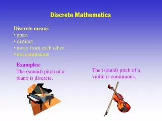
R. Johnsonbaugh, Discrete Mathematics. Chapter 4 Algorithms. 4.1 Introduction. An algorithm is a finite set of instructions with the following characteristics: Precision : steps are precisely stated

E N D
R. Johnsonbaugh,Discrete Mathematics Chapter 4 Algorithms
4.1 Introduction • An algorithm is a finite set of instructions with the following characteristics: • Precision: steps are precisely stated • Deterministic: Results of each step of execution are uniquely defined. They depend only on inputs and results of preceding steps • Finiteness: the algorithm stops after finitely many steps. • Correctness: The output produced is correct.
More characteristics of algorithms • Input: the algorithm receives input • Output: the algorithm produces output • Generality: the algorithm applies to various sets of inputs
Example: a simple algorithm Algorithm to find the largest of three numbers a, b, c: Assignment operator s := k means “copy the value of k into s” 1. x:= a 2. If b > x then x:= b 3. If c > x then x:= c A trace is a check of the algorithm for specific values of a, b and c
Pseudocode: Instructions given in a generic language similar to a computer language such as C++ or Pascal. procedure if-then, action if-then-else begin return while loop for loop end 4.2 Examples of algorithms
Variable declaration integer x, y; real x; or x : integer; boolean a; char c, d; datatype x; Note: We shall prefer not to give a complete declaration when the context of variables is obvious.
Assignment statements x := expression; or x = expression; or x expression; eg. x 1 + 3 *2 y := a * y + 2;
Control structures • if if <condition> then <a sequence of statements> [else <a sequence of statements>] endif
Control structures (cont.) • While while <condition> do <statements>; endwhile
Control structures (cont.) • loop-until loop <statements>; until < condition> Note: In comparison to while statement, the loop-until guarantees that the <statements> will be executed at least once.
Control structures (cont.) • for for i = <n1> to <n2> [step d] <statements> endfor
Control structures (cont.) • Case case : <condition1> : <statements1>; <condition2> : <statements2>; : <conditionn> : <statementsn>; [default : <statements>] endcase
I/O statements read(<argument list>); print(<argument list>);
Exit statement Example while condition1 do while condition2 do while condition3 do if…then exit (exit from the outmost loop) endwhile endwhile endwhile
Functions and procedures function name(parameter list) begin declarations statements; return(value); endname
Functions and procedures procedure name(parameter list) begin declarations statements; endname Note: Procedures are the similar to functions but they have no return statement.
Examples Procedure swap( x, y) /* in this case x, y are inout*/ begin temp x x y y temp endswap
Examples: Find the maximum value of 3 numbers Input: a, b, c Output: large (the largest of a, b, and c) procedure max(a,b,c) { large = a if (b > large) large = b if (c > large) large = c return large }
Examples: Find the maximum value in a sequence S1, S2, S3,…, Sn Input: S, n Output: large (the largest value in the sequence S) procedure max(S,n) { large = S1 for i = 2 to n if (Si > large) large = Si return large }
Examples: Print the even numbers 2, 4, 6,…, 10 Input: None Output: even numbers 2, 4, 6,…, 10 procedure printEven() { for i = 2 to 10 print i; }
Examples: Read 10 integer values, sort them in ascending order and print the even numbers Input: None Output: Sorted 10 integer values in ascending order procedure simpleSort() { integer numbers[10] for i = 1 to 10 read numbers[i];
Examples: Read 10 integer values, sort them in ascending order and print the even numbers for i = 1 to 10 { for j = i+1 to 10 { if (numbers[i] > numbers[j] ) then { temp = numbers[i] numbers[i] = numbers[j] numbers[j] = temp } } }
Examples: Read 10 integer values, sort them in ascending order and print the even numbers for i = 1 to 10 print numbers[i]; }
4.3 Analysis of algorithms • Big O notation Definition: f(n) = O(g(n)) iff there exist two positive constants c and n0 such that |f(n)| <= c |g(n)| for all n >= n0. Theorem If A(n) = am nm +…+ a1n + a0 is a polynomial of degree m then A(n) = O(nm).
Analysis of algorithms Ex. f(n) = 3 n2 f(n) = O(n2) Ex. f(n) = 3 n2 + 5n + 4 f(n) = O(n2)
4.4 Recursive algorithms • A recursive procedure is a procedure that invokes itself • Example: given a positive integer n, factorial of n is defined as the product of n by all numbers less than n and greater than 0. Notation: n! = n(n-1)(n-2)…3.2.1 • Observe that n! = n(n-1)! = n(n-1)(n-2)!, etc. • A recursive algorithm is an algorithm that contains a recursive procedure
Fibonacci sequence • Leonardo Fibonacci (Pisa, Italy, ca. 1170-1250) • Fibonacci sequence f1, f2,… defined recursively as follows: f1 = 1 f2 = 2 fn = fn-1 + fn-2 for n > 3 • First terms of the sequence are: 1, 2, 3, 5, 8, 13, 21, 34, 55, 89, 144, 233, 377, 610, 987, 1597,…
How to write a recursion algorithm Function a(input) begin basis steps; /* for minimum size input */ call a(smaller input); /* could be a number of recursive calls*/ combine the sub-solution of the recursive call; end a
Recursion (cont.) function max( A[i : j]) begin if i = j then return( A[i]); else m1 = max ( A[ i : (i+j)/2] ); m2 = max ( A[ (i+j)/2 + 1 : j] ); if m1 > m2 then return( m1) else return(m2) endif endif endmax
Recursion: 4 Basic Rules • Base cases can be solved without recursion. • Making progress toward a base case for cases that are to be solved recursively.
Recursion: 4 Basic Rules • Design rule. Assume that all recursive calls work. • Compound interest rule. Never duplicate work by solving the same instance of a problem in separate recursive calls.
Recursion: A poor use of recursion fib (int : n) begin if ( n <= 1) then return 1; else return fib(n-1) + fib(n-2) /*redundant work*/ endif end fib
Complexity: the amount of time and/or space needed to execute the algorithm. Complexity depends on many factors: data representation type, kind of computer, computer language used, etc. 4.5 Complexity of algorithms
Types of complexity • Best-case time = minimum time needed to execute the algorithm for inputs of size n • Worst-case time = maximum time needed to execute the algorithm for inputs of size n • Average-case time = average time needed
Order of an algorithm Let f and g be functions with domain Z+ = {1, 2, 3,…} • f(n) = O(g(n)): f(n) is of order at most g(n) • if there exists a positive constant C1 such that |f(n)| < C1|g(n)| for all but finitely many n • f(n) = (g(n)): f(n) is of order at least g(n) • if there exists a positive constant C2 such that |f(n)| > C2|g(n)| for all but finitely many n • f(n) = (g(n)): f(n) is or order g(n) if it is O(g(n)) and (g(n)).
Review of Big O Example: 3n + 2 = O(n) as 3n + 2 <= 4n for all n >= 2. 3n + 3 = O(n) as 3n + 3 <= 4n for all n >= 3. 100n + 6 = O(n) as 100n + 6 <= 101n for all n >= 10. 10n2 + 4n + 2 = O(n2) as 10n2 + 4n + 2 <= 11 n2 for n>= 5. 3n + 2 is not O(1) as 3n + 2 is not less than or equal to c or any constant c for all n.
Review of Big O • O-notation is a means for describing an algorithm’s performance. • O-notation is used to express an upper bound on the value of f(n). • O-notation doesn’t say how good the bound is.
Review of Big O • Notice that n = O(n2), n = O(n3), n = O(2n) etc. In order for the statement f(n) = O(n) to be informative, g(n) should be the as small a function of n as one can come up. We shall never say 3n + n = O(n2) even though it’s correct.
Review of Big O • f(n) = O(g(n)) is not the same as O(g(n)) = f(n).
Review of 3n + 2 =(n) as 3n + 2 >= 3n for all n >= 1. 3n + 3 = (n) as 3n + 3 >= 3n for all n >= 1. 100n + 6 = (n) as100n + 6 >= 100n for all n >= 1. 10n2 + 4n + 2 = (n2) as 10n2 + 4n + 2 >= n2 for n>= 1. 3n + 2 is not O(1) as 3n + 2 is not less than or equal to c or any constant c for all n.
Review of q 3n + 2 = q(n) as 3n + 2 >= 3n for all n >= 1 and 3n + 2 <= 4n for all n >= 2 so c1 = 3 and c2 = 4 and n0 = 2 Note: The theta is more precise than both the big O and omega notations.
Review of notations Notice that the coefficients in all the g(n) used have been 1. This is accordance with practice. We shall never find ourselves saying that 3n + 3 = O(4n), or that 10 = O(100) even though each of these statements is true.