FACTOR MODELS (Chapter 6)

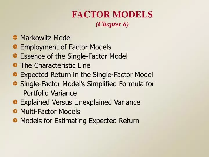
1. FACTOR MODELS(Chapter 6) • Markowitz Model • Employment of Factor Models • Essence of the Single-Factor Model • The Characteristic Line • Expected Return in the Single-Factor Model • Single-Factor Model’s Simplified Formula for Portfolio Variance • Explained Versus Unexplained Variance • Multi-Factor Models • Models for Estimating Expected Return

2. Markowitz Model Problem: Tremendous data requirement. • Number of security variances needed = M. • Number of covariances needed = (M2 - M)/2 • Total = M + (M2 - M)/2 • Example: (100 securities) • 100 + (10,000 - 100)/2 = 5,050 • Therefore, in order for modern portfolio theory to be usable for large numbers of securities, the process had to be simplified. (Years ago, computing capabilities were minimal)

3. Employment of Factor Models • To generate the efficient set, we need estimates of expected return and the covariances between the securities in the available population. Factor models may be used in this regard. • Risk Factors – (rate of inflation, growth in industrial production, and other variables that induce stock prices to go up and down.) • May be used to evaluate covariances of return between securities. • Expected Return Factors – (firm size, liquidity, etc.) • May be used to evaluate expected returns of the securities. • In the discussion that follows, we first focus on risk factor models. Then the discussion shifts to factors affecting expected security returns.

4. Essence of the Single-Factor Model • Fluctuations in the return of a security relative to that of another (i.e., the correlation between the two) do not depend upon the individual characteristics of the two securities. Instead, relationships (covariances) between securities occur because of their individual relationships with the overall market (i.e., covariance with the market). • IfStock (A) is positively correlated with the market, and ifStock (B) is positively correlated with the market, then Stocks (A) and (B) will be positively correlated with each other. • Given the assumption that covariances between securities can be accounted for by the pull of a single common factor (the market), the covariance between any two stocks can be written as:

5. The Characteristic Line(See Chapter 3 for a Review of the Statistics) • Relationship between the returns on an individual security and the returns on the market portfolio: • Aj= intercept of the characteristic line (the expected rate of return on stock (j) should the market happen to produce a zero rate of return in any given period). • j= beta of stock (j); the slope of the characteristic line. • j,t= residual of stock (j) during period (t); the vertical distance from the characteristic line.

6. Graphical Display of the Characteristic Line rj,t = j Aj rM,t

7. The Characteristic Line (Continued) • Note: A stock’s return can be broken down into two parts: • Movement along the characteristic line (changes in the stock’s returns caused by changes in the market’s returns). • Deviations from the characteristic line (changes in the stock’s returns caused by events unique to the individual stock). • Movement along the line: Aj + jrM,t • Deviation from the line: j,t

8. Major Assumption of the Single-Factor Model • There is no relationship between the residuals of one stock and the residuals of another stock (i.e., the covariance between the residuals of every pair of stocks is zero). Stock j’s Residuals (%) Stock k’s Residuals (%)

9. Expected Return in the Single-Factor Model • Actual Returns: • Expected Residual: • Given the characteristic line is truly the line of best fit, the sum of the residuals would be equal to zero • Therefore, the expected value of the residual for any given period would also be equal to zero: • Expected Returns: • Given the characteristic line, and an expected residual of zero, the expected return of a security according to the single-factor model would be:

10. Single-Factor Model’s Simplified Formula for Portfolio Variance • Variance of an Individual Security: • Given: • It Follows That:

11. Note: Therefore:

12. Variance of a Portfolio • Same equation as the one for individual security variance: • Relationship between security betas & portfolio betas • Relationship between residual variances of stocks, and the residual variance of a portfolio, given the index model assumption. The residual variance of a portfolio is a weighted average of the residual variances of the stocks in the portfolio with the weights squared.

13. Explained Vs. Unexplained Variance(Systematic Vs. Unsystematic Risk) • Total Risk = Systematic Risk + Unsystematic Risk • Systematic: That part of total variance which is explained by the variance in the market’s returns. • Unsystematic: The unexplained variance, or that part of total variance which is due to the stock’s unique characteristics.

14. Note: [i.e.,j22(rM)is equal to the coefficient of determination (the % of the variance in the security’s returns explained by the variance in the market’s returns) times the security’s total variance] Total Variance = Explained + Unexplained As the number of stocks in a portfolio increases, the residual variance becomes smaller, and the coefficient of determination becomes larger.

15. Explained Vs. Unexplained Variance(A Graphical Display) Coefficient of Determination Residual Variance Number of Stocks Number of Stocks

16. Explained Vs. Unexplained Variance(A Two Stock Portfolio Example) Covariance Matrix for Explained Variance Covariance Matrix for Unexplained Variance

17. Explained Vs. Unexplained Variance (A Two Stock Portfolio Example) Continued

18. A Note on Residual Variance • The Single-Factor Model assumes zero correlation between residuals: In this case, portfolio residual variance is expressed as: In reality, firms’ residuals may be correlated with each other. That is, extra-market events may impact on many firms, and: In this case, portfolio residual variance would be:

19. Markowitz Model Versus the Single-Factor Model (A Summary of the Data Requirements) • Markowitz Model • Number of security variances = m • Number of covariances = (m2 - m)/2 • Total = m + (m2 - m)/2 • Example - 100 securities: 100 + (10,000 - 100)/2 = 5,050 • Single-Factor Model • Number of betas = m • Number of residual variances = m • Plus one estimate of2(rM) • Total = 2m + 1 • Example - 100 securities: 2(100) + 1 = 201

20. Multi-Factor Models • Recall the Single-Factor Model’s formula for portfolio variance: If there is positive covariance between the residuals of stocks, residual variance would be high and the coefficient of determination would be low. In this case, a multi-factor model may be necessary in order to reduce residual variance. • A Two Factor Model Example where: rg = growth rate in industrial production rI = % change in an inflation index

21. Two Factor Model Example - Continued • Once again, it is assumed that the covariance between the residuals of the the individual stocks are equal to zero: • Furthermore, the following covariances are also presumed: • Portfolio Variance in a Two Factor Model:

22. where: Note that if the covariances between the residuals of the individual securities are still significantly different from zero, you may need to develop a different model (perhaps a three, four, or five factor model).

23. Note on the Assumption Cov(rg,rI ) = 0 • If the Cov(rg,rI) is not equal to zero, the two factor model becomes a bit more complex. In general, for a two factor model, the systematic risk of a portfolio can be computed using the following covariance matrix: To simplify matters, we will assume that the factors in a multi-factor model are uncorrelated with each other. I,p g,p g,p I,p

24. Models for Estimating Expected Return • One Simplistic Approach • Use past returns to predict expected future returns. Perhaps useful as a starting point. Evidence indicates, however, that the future frequently differs from the past. Therefore, “subjective adjustments” to past patterns of returns are required. • Systematic Risk Models • One Factor Systematic Risk Model: Given a firm’s estimated characteristic line and an estimate of the future return on the market, the security’s expected return can be calculated.

25. Models for Estimating Expected Return(Continued) • Two Factor Systematic Risk Model: • N Factor Systematic Risk Model: • Other Factors That May Be Used in Predicting Expected Return • Note that the author discusses numerous factors in the text that may affect expected return. A review of the literature, however, will reveal that this subject is indeed controversial. In essence, you can spend the rest of your lives trying to determine the “best factors” to use. The following summarizes “some” of the evidence.

26. Other Factors That May Be Used in Predicting Expected Return • Liquidity (e.g., bid-asked spread) • Negatively related to return [e.g., Low liquidity stocks (high bid-asked spreads) should provide higher returns to compensate investors for the additional risk involved.] • Value Stock Versus Growth Stock • P/E Ratios • Low P/E stocks (value stocks) tend to outperform high P/E stocks (growth stocks). • Price/(Book Value) • Low Price/(Book Value) stocks (value stocks) tend to outperform high Price/(Book Value) stocks (growth stocks).

27. Other Factors That May Be Used in Predicting Expected Return (continued) • Technical Analysis • Analyze past patterns of market data (e.g., price changes) in order to predict future patterns of market data. “Volumes have been written on this subject. • Size Effect • Returns on small stocks (small market value) tend to be superior to returns on large stocks. Note: Small NYSE stocks tend to outperform small NASDAQ stocks. • January Effect • Abnormally high returns tend to be earned (especially on small stocks) during the month of January.

28. Other Factors That May Be Used in Predicting Expected Return (continued) • And the List Goes On • If you are truly interested in factors that affect expected return, spend time in the library reading articles in Financial Analysts Journal, Journal of Portfolio Management, and numerous other academic journals. This could be an ongoing venture the rest of your life.

29. Building a Multi-Factor Expected Return Model: One Possible Approach • Estimate the historical relationship between return and “chosen” variables. Then use this relationship to predict future returns. • Historical Relationship: • Future Estimate:

30. Using the Markowitz and Factor Modelsto Make Asset Allocation Decisions • Asset Allocation Decisions • Portfolio optimization is widely employed to allocate money between the major classes of investments: • Large capitalization domestic stocks • Small capitalization domestic stocks • Domestic bonds • International stocks • International bonds • Real estate

31. Using the Markowitz and Factor Modelsto Make Asset Allocation Decisions Continued:Strategic Versus Tactical Asset Allocation • Strategic Asset Allocation • Decisions relate to relative amounts invested in different asset classes over the long-term. Rebalancing occurs periodically to reflect changes in assumptions regarding long-term risk and return, changes in the risk tolerance of the investors, and changes in the weights of the asset classes due to past realized returns. • Tactical Asset Allocation • Short-term asset allocation decisions based on changes in economic and financial conditions, and assessments as to whether markets are currently underpriced or overpriced.

32. Using the Markowitz and Factor Modelsto Make Asset Allocation Decisions Continued • Markowitz Full Covariance Model • Use to allocate investments in the portfolio among the various classes of investments (e.g., stocks, bonds, cash). Note that the number of classes is usually rather small. • Factor Models • Use to determine which individual securities to include in the various asset classes. The number of securities available may be quite large. Expected return factor models could also be employed to provide inputs regarding expected return into the Markowitz model. • Further Information • Interested readers may refer to Chapter 7, Asset Allocation, for a more indepth discussion of this subject. In addition, the author has provided “hands on” examples of manipulating data using the PManager software in the process of making asset allocation decisions.