Download
1 / 44
450 likes | 753 Views
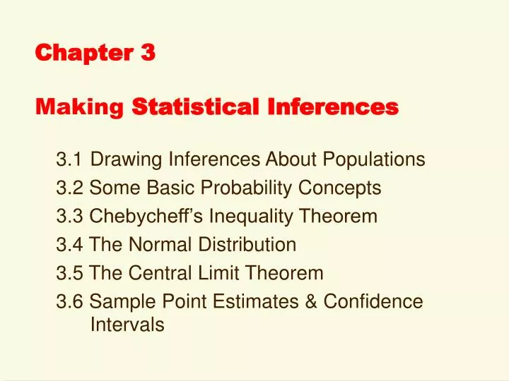
Chapter 3 Making Statistical Inferences. 3.1 Drawing Inferences About Populations 3.2 Some Basic Probability Concepts 3.3 Chebycheff’s Inequality Theorem 3.4 The Normal Distribution 3.5 The Central Limit Theorem 3.6 Sample Point Estimates & Confidence Intervals.

E N D
Chapter 3Making Statistical Inferences 3.1 Drawing Inferences About Populations 3.2 Some Basic Probability Concepts 3.3 Chebycheff’s Inequality Theorem 3.4 The Normal Distribution 3.5 The Central Limit Theorem 3.6 Sample Point Estimates & Confidence Intervals
Inference - from Sample to Population Inference: process of making generalizations (drawing conclusions) about a population’s characteristics from the evidence in one sample To make valid inferences, a representative sample must be drawn from the population using SIMPLE RANDOM SAMPLING • Every population member has equal chance of selection • Probability of a case selected for the sample is 1/Npop • Every combination of cases has same selection likelihood We’ll treat GSS as a s.r.s., altho it’s not
Probability Theory In 1654 the Chevalier de Méré, a wealthy French gambler, asked mathematician Blaise Pascal if he should bet even money on getting one “double six” in 24 throws of two dice? Pascal’s answer was no, because the probability of winning is only .491. The Chevalier’s question started an famous exchange of seven letters between Pascal and Pierre de Fermat in which they developed many principles of the classical theory of probability. A Russian mathematician, Andrei Kolmogorov, in a 1933 monograph, formulated the axiomatic approach which forms the foundation of the modern theory of probability. Pascal Fermat
Sample Spaces A simplechanceexperiment is a well-defined act resulting in a single event; for example, rolling a die or cutting a card deck. This process is repeatable indefinitely under identical conditions, with outcomes assumed equiprobable (equally likely to occur). To compute exact event probabilities, you must know an experiment’s sample space (S), the set (collection) of all possible outcomes. The theoretical method involves listing all possible outcomes. For rolling one die: S = {1, 2, 3, 4, 5, 6}. For tossing two coins, S = {HH, HT, TH, TT}. Probability of an event: Given sample space S with a set of E outcomes, a probability function assigns a real number p(Ei) to each event iin the sample space.
Axioms & Theorems Three fundamental probability axioms (general rules): 1. The probability assigned to event i must be a nonnegative number: p(Ei) > 0 2. The probability of the sample space S (the collection of all possible outcomes) is 1: p(S) = 1 3. If two events can't happen at the same time, then the probability that either event occurs is the sum of their separate probabilities: p(E1) or p(E2)=p(E1) + p(E2) Two important theorems (deductions) can be proved: 1. The probability of the empty (“impossible”) event is 0: p(E0) = 0 2. The probability of any event must lie between 0 and 1, inclusive: 1 > p(Ei) > 0
Calculate these theoretical probabilities: For rolling a single die, calculate the theoretical probability of a “4”: _______________ Of a “7”: _______________ 1/6 = .167 0/6 = .000 For a single die roll, calculate the theoretical probability of getting either a “1” or “2” or “3” or “4” or “5” or “6”: ______________________________________________ 1/6 + 1/6 + 1/6 + 1/6 + 1/6 + 1/6 = 6/6 = 1.00 For tossing two coins, what is the probability of two heads: ________ Of one head and one tail: ________ .250 .500 If you cut a well-shuffled 52-card deck, what is the probability of getting the ten of diamonds? ____________ What is the probability of any diamond card? ____________ .0192 .250
Relative Frequency An empirical alternative to the theoretical approach is to perform a chance experiment repeatedly and observe outcomes. Suppose you roll two dice 50 times and find these sums of their face values. What are the empirical probabilities of seven? four? ten? FIFTY DICE ROLLS 4 10 6 7 5 10 4 6 5 6 11 12 3 3 6 7 10 10 4 4 7 8 8 7 7 4 10 11 3 8 6 10 9 4 8 4 3 8 7 3 7 5 4 11 9 5 2 5 8 5 In therelative frequencymethod, probability is the proportion of times that an event occurs in a “large number” of repetitions: 7/50 = .14 p(E7) = _________ p(E4) = _________ p(E10) = ________ 8/50 = .16 6/50 = .12 But, theoretically seven is the most probable sum (.167), while four and ten each have much lower probabilities (.083). Maybe this experiment wasn’t repeated often enough to obtain precise estimates? Or were these two dice “loaded?” What do we mean by “fair dice?”
Interpretation • Despite probability theory’s origin in gambling, relative frequency remains the primary interpretation in the social sciences. If event rates are unknowable in advance, a “large N” of sample observations may be necessary to make accurate estimates of such empirical probabilities as: • What is the probability of graduating from college? • How likely are annual incomes of $100,000 or more? • Are men or women more prone to commit suicide? • Answers require survey or census data on these events. Don’t confuse formal probability concepts with everyday talk, such as “John McCain will probably be elected” or “I probably won’t pass tomorrow’s test.” Such statements express only a personal belief about the likelihood of a unique event, not an experiment repeated over and over.
Describing Populations Population parameter: a descriptive characteristic of a population such as its mean, variance, or standard deviation • Latin = sample statistic • Greek = population parameter Box 3.1 Parameters & Statistics
3.3 Chebycheff's Inequality Theorem If you have the book, read this subsection (pp. 73-75) as background information on the normal distribution. Because Cheby’s inequality is never calculated in research statistics, we’ll not spend time on it in lecture.
The Normal Distribution Normal distribution: smooth, bell-shaped theoretical probability distribution for a continuous variable, generated by a formula: where e is Euler’s constant (= 2.7182818….) The population mean and variance determine a particular distribution’slocation and shape. Thus, the family of normal distributions has an infinite number of curves.
Comparing Three Normal Curves Suppose we graph three normally distributions, each with a mean of zero: (Y = 0) What happens to the height and spread of these normal probability distributions if we increase the population’s variance? Next graph superimposes these three normally distributed variables with these variances: (1) = 0.5 (2) = 1.0 (3) = 1.5
Standardizing a Normal Curve To standardize any normal distribution, change the Y scores to Z scores, whose mean = 0 and std. dev. = 1. Then use the known relation between the Z scores and probabilities associated with areas under the curve. We previously learned how to convert a sample of Yi scores into standardized Zi scores: Likewise, we can standardize a population of Yi scores: We can use a standardized Z score table (Appendix C) to solve all normal probability distribution problems, by finding the area(s) under specific segment(s) of the curve.
Area = Probability The TOTAL AREA under a standardized normal probability distribution is assumed to have unit value; i.e., = 1.00 This area corresponds to probability p = 1.00 (certainty). Exactly half the total area lies on each side of the mean, (Y = 0) (left side negative Z, right side positive Z) Thus, each half of the normal curve corresponds to p = 0.500
Areas Between Z Scores Using the tabled values in a table, we can find an area (a probability) under a standardized normal probability distribution that falls between two Z scores EXAMPLE #1: What is area between Z = 0 and Z = +1.67? EXAMPLE #2: What is area from Z = +1.67 to Z = +? 0 +1.67 Also use the Web-page version of Appendix C, which gives pairs of values for the areas (0 to Z) and (Z to ).
Appendix C The Z Score Table Z score Area from 0 to Z Area from Z to ∞ 1.50 0.4332 0.0668 … 1.60 0.4452 0.0548 … 1.65 0.4505 0.0495 1.66 0.4515 0.0485 1.67 0.4525 0.0475 1.68 0.4535 0.0465 1.69 0.4545 0.0455 1.70 0.4554 0.0446 For Z = 1.67: Col. 2 = __________ Col. 3 = __________ Sum = __________ 0.4525 0.0475 0.5000 EX #3: What is area between Z = 0 and Z = -1.50? 0.4332 EX #4: What is area from Z = -1.50 to Z = -? 0.0668
Calculate some more Z score areas 0.0495 EX #5: Find the area from Z = -1.65 to - _________ 0.0250 EX #6: Find the area from Z = +1.96 to _________ 0.0099 EX #7: Find the area from Z = -2.33 to - _________ 0.4951 EX#8: Find the area from Z = 0 to –2.58 _________ Use the table to locate areas between or beyond two Z scores. Called“two-tailed” Z scoresbecause areas are inboth tails: 0.9500 EX #9: Find the area from Z = 0 to 1.96 _________ 0.0500 EX #10: Find the areas from Z = 1.96 to _________ 0.0098 EX #11: Find the areas from Z = 2.58 to _________
The Useful Central Limit Theorem Central limit theorem:if all possible samples of size N are drawn from any population, with mean and variance , then as N grows large, the sampling distribution of these means approaches a normal curve, with mean and variance The positive square root of a sampling distribution’s variance (i.e., its standard deviation), is called thestandard errorof the mean:
Take ALL Samples in a Small Population Population (N = 6, mean = 4.33): Form all samples of size n = 2 & calculate means: Y1+Y2 = (2+2)/2 = 2 Y1+Y3 = (2+4)/2 = 3 Y1 = 2 Y2 = 2 Y3 = 4 Y4 = 4 Y5 = 6 Y6 = 8 Y1+Y5 = (2+6)/2 = 4 Y1+Y4 = (2+4)/2 = 3 Y2+Y3 = (2+4)/2 = 3 Y1+Y6 = (2+8)/2 = 5 Y2+Y5 = (2+6)/2 = 4 Y2+Y4 = (2+4)/2 = 3 Y3+Y4 = (4+4)/2 = 4 Y2+Y6 = (2+8)/2 = 5 Y3+Y6 = (4+8)/2 = 6 Y3+Y5 = (4+6)/2 = 5 Y4+Y6 = (4+8)/2 = 6 Y4+Y5 = (4+6)/2 = 5 Y5+Y6 = (6+8)/2 = 7 Calculate the mean of these 15 sample means = ___________ 4.33 Graph this sampling distribution of 15 sample means: Probability that a sample mean = 7? ______________________ 1 in 15: p = 0.067 2 3 4 5 6 7
Take ALL Samples in a Large Population A “thought experiment” suggests how a theoretical sampling distribution is built by: (a) forming every sample of size N in a large population, (b) then graphing all samples’ mean values. Let’s take many samples of 1,000 persons and calculate each sample’s mean years of education: A graph of this sampling distribution of sample means increasingly approaches a normal curve: #1 mean = 13.22 Population #2 mean = 10.87 #100 mean = 13.06 8 9 10 11 12 13 14 15 16 17 #1000 mean = 11.59
Sampling Distribution for EDUC Start with a variable in a population with a known standard deviation: U.S. adult population of about 230,000,000 has a mean education = 13.43 years of schooling with a standard deviation = 3.00. If we generate sampling distributions for samples of increasingly larger N, what do you expect will happen to the values of the mean and standard error for these sampling distributions, according to the Central Limit Theorem?
Sampling distributions with differing Ns 1. Let’s start with random samples of N = 100 observations. CAUTION! BILLIONS of TRILLIONS of such small samples make up this sampling distribution!!! What are the expected values for mean & standard error? 13.43 0.300 2. Now double N = 200. What mean & standard error? 13.43 0.212 3. Use GSS N = 2,018. What mean & standard error? 13.43 0.067
Online Sampling Distribution Demo Rice University Virtual Lab in Statistics: http://onlinestatbook.com/stat_sim/ Choose & clickSampling Distribution Simulation (requires browser with Java 1.1 installed) Read Instructions, Click ”Begin” button We’ll work some examples in class, then you can try this demo for yourself. See screen capture on next slide:
How Big is a “Large Sample?” • To be applied, the central limit theorem requires a “large sample” • But how big must a simple random sample be for us to call it “large”? SSDA p. 81: “we cannot say precisely.” • N < 30 is a “small sample” • N > 100 is a “large sample” • 30 < N < 100 is indeterminate
The Alpha Area Alpha area ( area): area in tail of normal distribution that is cut off by a given Z Because we could choose to designate in either the negative or positive tail (or in both tails, by dividing in half), we define an alpha area’s probability using the absolute value: p(|Z| |Z|) = Critical value (Z): the minimum value of Z necessary to designate an alpha area
Find the critical values of Z that define six alpha areas: 1.65 2.33 3.10 Z = ________ Z = ________ Z = ________ = 0.05 one-tailed = 0.01 one-tailed = 0.001 one-tailed ±1.96 ±2.58 ±3.30 Z = ________ Z = ________ Z = ________ = 0.05 two-tailed = 0.01 two-tailed = 0.001 two-tailed These and Z are the six conventional values used to test hypotheses.
Apply Z scores to a sampling distribution of EDUC where What is the probability of selecting a GSS sample of N = 2,018 cases whose mean is equal to or greater than 13.60? C: Area Beyond Z = _____________ +2.54 0.0055 What is the probability of drawing a sample with mean = 13.30 or less? C: Area Beyond Z = ______________ -1.94 0.0262
Two Z Scores in a Sampling Distribution Z = -1.94 Z = +2.54 p = .0055 p = .0262
Find Sample Means for an Alpha Area What sample means divide = .01 equally into both tails of the EDUC sampling distribution? /2 = (.01)/2 = .005 1. Find half of alpha: 2. Look up the two values of the critical Z/2scores: In Table C the area beyond Z ( = .005), Z/2=_________ 2.58 3. Rearrange Z formula to isolate the sample mean on one side of the computation: (+2.58)(0.067)+13.43 = 13.60 yrs (-2.58)(0.067)+13.43 = 13.26 yrs 4. Compute the two ___________________________________ critical mean values:___________________________________
Point Estimate vs. Confidence Interval Point estimate:sample statistic used to estimate a population parameter In the 2008 GSS, mean family income = $58,683, the standard deviation = $46,616 and N = 1,774. Thus, the estimated standard error = $46,616/42.1 = $1,107. Confidence interval: a range of values around a point estimate, making possible a statement about the probability that the population parameter lies between upper and lower confidence limits The 95% CI for U.S. annual income is from $56,513 to $60,853, around a point estimate of $58,683. Below you will learn below how use the sample mean and standard error to calculate the two CI limits.
Confidence Intervals An important corollary of the central limit theorem is that the sample mean is the best point estimateof the mean of the population from which the sample was drawn: We can use the sampling distribution’s standard error to build a confidence interval around a point-estimated mean. This interval is defined by the upper and lower limits of its range, with the point estimate at the midpoint. Then use this estimated interval to state how confident you feel that the unknown population parameter (Y) falls inside the limits defining the interval.
UCL & LCL A researcher sets a confidence interval by deciding how “confident” she wishes to be. The trade-off is that obtaining greater confidence requires a broader interval. • Select an alpha (α) for desired confidence level • Split alpha in half (α/2) & find the critical Z scores in the standardized normal table (+ and – values) • Multiply each Zα/2 by the standard error, then separately add each result to sample mean Upper confidence limit, UCL: Lower confidence limit, LCL:
Show how to calculate the 95% CI for 2008 GSS income For GSS sample N = 1,774 cases, sample mean: The standard error for annual income: Upper confidence limit, 95% UCL: $58,683 + (1.96)($1,107) = $58,683 + $2,170 = $60,853 Lower confidence limit, 95% LCL: $58,683 - (1.96) ($1,107) = $58,683 - $2,170 = $56,513 Now compute the 99% CI: Upper confidence limit, 99% UCL: $58,683 + (2.58) ($1,107) = $58,683 + $2,856 = $61,539 Lower confidence limit, 99% LCL: $58,683 - (2.58) ($1,107) = $58,683 - $2,856 = $55,827
For find the UCL & LCL for these two CIs: A:The 95% confidence interval: = 0.05, so Z = 1.96 UCL = 40 + 11.76 = 51.76 LCL = 40 - 11.76 = 28.24 B: The 99% confidence interval; = 0.01, so Z = 2.58 UCL = 40 + 15.48 = 55.48 LCL = 40 - 15.48 = 24.52 Thus, to obtain more confidence requires a wider interval.
Interpretating a CI A CI interval indicates how much uncertainty we have about a sample estimate of the true population mean. The wider we choose an interval (e.g., 99% CI), the more confident we are. CAUTION: A 95% CI does not mean that an interval has a 0.95 probability of containing the true mean. Any interval estimated from a sample either contains the true mean or it does not – but you can’t be certain! Correct interpretation: A confidence interval is not a probability statement about a single sample, but is based on the idea of repeated sampling. If all samples of the same size (N) were drawn from a population, and confidence intervals calculated around every sample mean, then 95% (or 99%) of intervals would be expected to contain the population mean (but 5% or 1% of intervals would not). Just say:“I’m 95% (or 99%) confident that the true population mean falls between the lower and upper confidence limits.”
Calculate another CI example If find UCL & LCL for two CIs: LCL = 50 - 6.2 = 43.8 UCL = 50 + 6.2 = 56.2 LCL = 50 - 8.2 = 41.8 UCL = 50 + 8.2 = 58.2 INTERPRETATION:For all samples of the same size (N), if confidence intervals were constructed around each sample mean, 95% (or 99%) of those intervals would include the population mean somewhere between upper and lower limits. Thus, we can be 95% confident that the population mean lies between 43.8 and 56.2. And we can have 99% confidence that the parameter falls into the interval from 41.8 to 58.2.
A Graphic View of CIs The confidence intervals constructed around 95% (or 99%) of all sample means of size N from a population can be expected to include the true population mean (dashed line) within the lower and upper limits. But, in 5% (or 1%) of the samples, the population parameter would fall outside their confidence intervals. μY
Online CI Demo Rice University Virtual Lab in Statistics: http://onlinestatbook.com/stat_sim/ Choose & clickConfidence Intervals (requires browser with Java 1.1 installed) Read Instructions, Click ”Begin” button We’ll work some examples in class, then you can try this demo for yourself. See screen capture on next slide:
What is a “Margin of Error”? Opinion pollsters report a “margin of error” with their point estimates: The Gallup Poll’s final survey of 2009, found that 51% of the 1,025 respondents said they approved how Pres. Obama was doing his job, with a margin of sampling error = ±3 per cent. Using your knowledge of basic social statistics, you can calculate -- (1) thestandard deviationfor the sample point-estimate of a proportion: (2) Use that sample value to estimate thesampling distribution’sstandard error: (3) Then find the upper and lower95% confidence limits: Thus, a “margin of error” is just the product of the standard error times the critical value of Z/2 for the 95% confidence interval!