Download
1 / 28
280 likes | 471 Views
Examining the Evolutionary Sequence of Massive Stars. Tracey Hill (UNSW/ATNF) Collaborators: Michael Burton (UNSW), Maria Hunt (UNSW), Jim Caswell (ATNF), Vincent Minier (CEA), Andrew Walsh (UNSW), Mark Thompson (UHerts). The study of Massive Stars. Why? We are made of star dust

E N D
Examining the Evolutionary Sequence of Massive Stars Tracey Hill (UNSW/ATNF) Collaborators: Michael Burton (UNSW), Maria Hunt (UNSW), Jim Caswell (ATNF), Vincent Minier (CEA), Andrew Walsh (UNSW), Mark Thompson (UHerts). Joint Astronomy Centre
The study of Massive Stars • Why? • We are made of star dust • The death and birth of stars may be linked. • Complex molecules can form on dust grains • Young stars “stir up” clouds of gas • Stars often harbour planets • Evolution not well understood • CEDAR • Optically obscured by circumstellar dust prior to MS • HOW? • Associated with: IRAS pt sources, UC HII, maser emission, mid-IR (MSX), sub-mm, mm
Evolution of a Massive Star CH3OH OH H20 Cold Hot GMC Core Molecular UC HII HII Core SED mm Mid IR Near IR Molecular lines evolving (?)
Aims of my thesis • To undertake a multi-wavelength study of star formation from the mid-IR to mm. • From this determine the SED from mid-IR to mm for a range of sources. • To propose an evolutionary sequence for MSF. • To determine the dust grain properties of MSF regions. (mm and sub-mm) • To determine the significance in fluctuations of the dust grain emissivity exponent ().
Results (SEST) • Targeted known positions of methanol masers and UC HII regions (129) using SIMBA. • 404 sources (3- detection limit). • 100% of sources targeted have mm continuum emission. +20 others in fields. • In the majority of sources, the position of the tracer targeted correlates with the peak millimetre emission. • Evidence of methanol masers and UC HII regions devoid of millimetre continuum emission. – Implications? • Evidence of star formation devoid of methanol masers and/or UC HII regions (“mm-only cores”) – Implications? • Other Data: • ATCA (3mm) on few cores. Resolving bright SIMBA • JCMT, fallback observations (Sept03), CS line data (Aug04) collaborators data, time allocated in Semester 05 A.
Sources targeted:- mm-continuum sources with no tracers. Are these sources at an earlier evolutionary sequence prior to the onset of methanol masers? To be tested with SEDs and dust emissivity exponent. SCUBA data
Introducing the ‘mm-only’ core • ~ 60% sources (253/404) detected have no maser &/or UC HII (mm-emission only). mm-only core • Readily detectable at sub-mm wavelengths. • Sept 03 JCMT data, showed 100% detection. • Time allocated to observe JCMT 05A (April?) • ~ 50 % do not have mid-IR MSX emission. [lower limit] or are devoid of a mid-IR source. • What is their story? • Younger? Deeply embedded? Intermediate mass? combination?
Ionized Core (UCHII region) Hot Molecular Core Cold Core A Range of MSF Cores1.2mm Continuum, SEST/SIMBA CH3CN HCN hanol HCO+ CH3OH (Reverse) Evolutionary Order?? Minier, Purcell, Hill et al, 2004
Data Analysis • 4 classes of source: (diff. evolutions?) • mm-only (mm), maser (mas), maser and radio (mr), radio (rad). • Assumed near distance to all with an ambiguity • 12 have no known distance. • Parameter analysis: • Mass, radius, H2 number density (nH2) • Kolmogorov-Smirnov testing (K-S testing). • Cumulative plots of mass for each distribution. • Histogram plots of each parameter • Correlation plots of parameters
Kolmogorov-Smirnov Testing • To test whether two distributions are drawn from the same distribution function. • Disproving the null-hypothesis proves that the data sets are from different distributions. • Failing to disprove the null-hypothesis shows that the data sets are consistent with a single distribution function. Null hypothesis = that the two groups are the same.
Cumulative plot of each distribution. Measures the maximum value of the absolute difference between two cumulative distribution functions. (it is the behaviour between the largest and smallest values that distinguishes a distribution). This is called the k-s statistic ‘D’. The Prob (P)of D > obs is calculated. The null hypothesis (that the two groups are the same) should be rejected if P is "small". How does K-S testing work?
Parameter: Mass • KS-test mm-only distributions are not from the same population as maser, mr, or radio. • maser and radio populations produce ‘D’ stat consistent with being related. [confirms work of Walsh et al and evol. seq. of MSF]
m r2.2 mm-only dominate low-mass low-radius end
Results - Summary • mm-only cores are smaller and less massive than cores with a maser and/or UC HII region. • mm-only cores have a range of masses consistent with those cores with tracers. • Mean mass mm-only: 0.9 x 10³ M • Mean mass masers + UC HII: 2.5 x 10³ M • mm-only cores have radii < 2.0 pc (bar one), with the majority (94%) < 1.0 pc. • Mean radius: 0.4 pc • Mean radius of masers + UC HII: 0.7 pc
Interpretation of the mm-only core • Precursor to the maser? • New class of source that represents the earliest stage of massive star formation prior to onset of maser emission. • Intermediate mass star formation? • Harbour protoclusters which do not contain any high mass stars (below HII limit). • Cross-section of sources supporting both arguments? • More massive mm-only cores support 1. • Less massive mm-only cores support 2. Hill et al. MNRAS 2005, submitted
Further Work Joint Astronomy Centre
Spectral Energy Distributions • The SED for each source is fitted using a two component grey-body function. • Models the emission from a warm dust core embedded in a larger cold envelope. • The SED is compiled using data spanning the MIR to the mm regime of the Electromagnetic spectrum. • MSX data at 8.3m, 12.1m, 14.6m, 21.3m. • Sub-mm data (SCUBA) at 450m and 850m. • mm data (SIMBA) at 1.2mm. • IRAS data (?) at 12-100m. • Reveals information relating to the source: • Temperature (leads to estimate of age, and hence ES) • Luminosity, density and calculation of mass.
Compiling a SED • From multi-Wavelength data to the SED:
The Dust Emissivity Exponent? • Tells us about the behaviour of the dust emissivity with wavelength (Dunne & Eales 2001). • Identifies the type of grain which makes up the central star forming core. • Ex. ~ 2 =crystalline grains, while ~1 = amorphous carbon grains, =2 for graphitic grains (Dunne & Eales 2001). • Ex. A value of = 1.5~2.0 is indicative of class 0 (collapsing protostar) sources (Furuya et al. ) • Ex. = 1.5 infers composite grains, while 0.6 1.4 infers fractal grains (Dunne & Eales 2001 and references within). • Sub-mm/mm emissivities are particularly important: • Molecules known to deplete inside protostellar cores. • Dust emissivity best tracer of gas density distribution just prior to onset of gravitational collapse. – i.e define the initial conditions from which a core collapses to form a star.
What does reveal? • The dust mass – the mass of the star forming cloud. • The star formation efficiency. • Can determine the dust-to-gas ratio (Hoare et al. 1991). • is complicated by: • Grain size, grain shape (assume spherical?), grain mixtures. (Hildebrand 1983). • Temperature (? in come cases), emissivity, and extinction with redshift and metallicity (Dunne & Eales 2001). • Not much work done observationally. • Most generally assume a value of when fitting the B/B fxn to data. • Computationally Ossenkopf and Henning (1994). • Hildebrand (1983), Dunne & Eales (2001). • Models and observations suggest that emissivities increase in dense cores (Ossenkopf & Henning 1994).
How do we determine ? F=c B where = (1-e-) F=c 2hc2/3 1/(ehc\kT –1) 0 (o/) Let A = c 2hc2o 0 , then: F= A/3 1/(ehc\kT –1) (1/) F= A/3+ 1/(ehc\kT –1) Fit function and derive
Assumptions (preliminary) • A 10% error assumed for all sub-mm and mm fluxes. • RJ-approx to B/B fxn. • Dealing with cold objects. • B/B fxn begins to break down. • However, 450m may not satisfy the RJ-approximation in all cases. • RJ-approx breaks down – hence, results incorrect.
Interpreting the results • Typically, values of fall between 1-2 • Some values are extreme ie. 0.4, 3.5 • This may be due to incorrect fluxes. • The fits themselves may not be robust. • Error contour plots show a high correlation between the gradient () and the y-intercept of the plots. • What is the significance (if any) in fluctuations of the dust emissivity exponent - ?
Future Work • SED compilation for all sources. • Determination and examination of beta • Compare with results determined theoretically (Ossenkopf & Henning, Dunne & Eales). • Indication of sturdiness of our results. • Interpretation of our results - what each beta value translates to in terms of grain properties. • Finish project and write up thesis.