Download
1 / 66

E N D
PH 0101 UNIT-3 LECTURE 7 • Fiber optics • Basic principles • Physical structure of optical fibre • Propagation characteristics of optical fibre PH 0101 UNIT 3 Lecture 8
Incident and refracted rays PH 0101 UNIT 3 Lecture 8
Refraction and Snell’s Law When a ray travels across a boundary between two materials with different refractive indices n1and n2, both refraction and reflection takes place. The case where n1 > n2; that is where the light travels from high to low refractive index materials. The refracted ray is “broken” that is, the angle 2 is not equal to 1. The relation between 1 and 2 is given by Snell’s law of refraction. (or) PH 0101 UNIT 3 Lecture 8
Total Internal reflection When 2, the angle of refraction becomes 90, the refracted beam is not traveling through the n2 material. Applying Snell’s law of refraction, The angle of incidence 1 for which 2= 90 is called the critical angle c: PH 0101 UNIT 3 Lecture 8
If the ray is incident on the boundary between n1 and n2 materials at the critical angle, the refracted ray will travel along the boundary, never entering the n2material. • There are no refracted rays for the case where • 1 >c. • This condition is known as total internal reflection, which can occur only when light travels from higher refractive index material to lower refractive index material. PH 0101 UNIT 3 Lecture 8
Refraction at the critical angle PH 0101 UNIT 3 Lecture 8
Light guides (a) Simple glass rod (b) Glass rod and cladding with different refraction qualities PH 0101 UNIT 3 Lecture 8
Propagation characteristics of optical fiber • Meridinal rays and Skew rays • The light rays, during the journey inside the optical fiber through the core, cross the core axis. Such light rays are known as meridinal rays. • The passage of such rays in a step index fiber is Similarly, the rays which never cross the axis of the core are known as the skew rays. • Skew rays describe angular ‘helices’ as they progress along the fiber. PH 0101 UNIT 3 Lecture 8
Meridinal rays Skew rays PH 0101 UNIT 3 Lecture 8
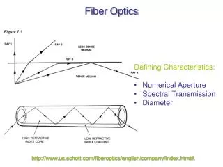
Acceptance Angle It should be noted that the fiber core will propagate the incident light rays only when it is incident at an angle greater than the critical angle c. The geometry of the launching of the light rays into an optical fiberis shown in Fig. PH 0101 UNIT 3 Lecture 8
Acceptance angle PH 0101 UNIT 3 Lecture 8
Numerical aperture A ray of light is launched into the fiber at an angle 1 is less than the acceptance angle a for the fiber as shown. PH 0101 UNIT 3 Lecture 8
The ray B entered at an angle greater than a and eventually lost propagation by radiation. • It is clear that the incident rays which are incident on fiber core within conical half angle a will be refracted into fiber core, propagate into the core by total internal reflection. • This angle a is called as acceptance angle, defined as the maximum value of the angle of incidence at the entrance end of the fiber, at which the angle of incidence at the core – cladding surface is equal to the critical angle of the core medium. PH 0101 UNIT 3 Lecture 8
Acceptance cone The imaginary light cone with twice the acceptance angle as the vertex angle, is known as the acceptance cone. Numerical Aperture (NA) Numerical aperture (NA) of the fiber is the light collecting efficiency of the fiber and is a measure of the amount of light rays can be accepted by the fiber. PH 0101 UNIT 3 Lecture 8
The half acceptance angle a is given by PH 0101 UNIT 3 Lecture 8
1. Calculate the numerical aperture and acceptance angle of fiber with a core index of 1.50 and a cladding index of 1.48. 2. Calculate the numerical aperture and acceptance angle of a optical fiber having core refractive index of 1.48 and relative index of 0.02. PH 0101 UNIT 3 Lecture 8
Classification of optical fibers Optical fibers are classified based on Material Number of modes and Refractive index profile PH 0101 UNIT 3 Lecture 8
Optical fibers based on material Optical fibers are made up of materials like silica and plastic. The basic optical fiber material must have the following properties: (i) Efficient guide for the light waves (ii) Low scattering losses (iii) The absorption, attenuation and dispersion of optical energy must be low. Based on the material used for fabrication, they are classified into two types: • Glass fibers and • Plastic fibers PH 0101 UNIT 3 Lecture 8
Glass fibers The glass fibers are generally fabricated by fusing mixtures of metal oxides and silica glasses. Silica has a refractive index of 1.458 at 850 nm. To produce two similar materials having slightly different indices of refraction for the core and cladding, either fluorine or various oxides such as B2O3, GeO2 or P2O3 are added to silica. Examples: SiO2 core; P2O3 – SiO2 cladding GeO2 – SiO2 core; SiO2 cladding P2O5 – SiO2 core; SiO2 cladding PH 0101 UNIT 3 Lecture 8
Plastic fibers • The plastic fibers are typically made of plastics and are of low cost. • Although they exhibit considerably greater signal attenuation than glass fibers, the plastic fibers can be handled without special care due to its toughness and durability. • Due to its high refractive index differences between the core and cladding materials, plastic fibers yield high numerical aperture and large angle of acceptance. PH 0101 UNIT 3 Lecture 8
Examples: • A polymethyl methacrylate core (n1 = 1.59) and a cladding made of its co-polymer (n2 = 1.40). • A polysterene core (n1 = 1.60) and a methylmetha crylate cladding (n2 = 1.49). PH 0101 UNIT 3 Lecture 8
Optical fibers based on modes or mode types • An optical fiber is a waveguide in the optical wavelength. • Mode is the one which describes the nature of propagation of electromagnetic waves in a wave guide. • i.e. it is the allowed direction whose associated angles satisfy the conditions for total internal reflection and constructive interference. • Based on the number of modes that propagates through the optical fiber, they are classified as: • Single mode fibers • Multi mode fibers PH 0101 UNIT 3 Lecture 8
Single mode fibers • In a fiber, if only one mode is transmitted through it, then it is said to be a single mode fiber. • A typical single mode fiber may have a core radius of 3 μm and a numerical aperture of 0.1 at a wavelength of 0.8 μm. • The condition for the single mode operation is given by the V number of the fiber which is defined as such that V ≤ 2.405. • Here, n1 = refractive index of the core; a = radius of the core; λ = wavelength of the light propagating through the fiber; Δ = relative refractive indices difference. PH 0101 UNIT 3 Lecture 8
The single mode fiber has the following characteristics: • Only one path is available. • V-number is less than 2.405 • Core diameter is small • No dispersion • Higher band width (1000 MHz) • Used for long haul communication • Fabrication is difficult and costly PH 0101 UNIT 3 Lecture 8
Single mode fiber Multi mode fiber PH 0101 UNIT 3 Lecture 8
Multi mode fibers • If more than one mode is transmitted through optical fiber, then it is said to be a multimode fiber. • The larger core radii of multimode fibers make it easier to launch optical power into the fiber and facilitate the end to end connection of similar powers. Some of the basic properties of multimode optical fibers are listed below: • More than one path is available • V-number is greater than 2.405 PH 0101 UNIT 3 Lecture 8
Core diameter is higher • Higher dispersion • Lower bandwidth (50MHz) • Used for short distance communication • Fabrication is less difficult and not costly Optical fibers based on refractive index profile Based on the refractive index profile of the core and cladding, the optical fibers are classified into two types: • Step index fiber • Graded index fiber. PH 0101 UNIT 3 Lecture 8
Step index fiber • In a step index fiber, the refractive index changes in a step fashion, from the centre of the fiber, the core, to the outer shell, the cladding. • It is high in the core and lower in the cladding. The light in the fiber propagates by bouncing back and forth from core-cladding interface. • The step index fibers propagate both single and multimode signals within the fiber core. • The light rays propagating through it are in the form of meridinal rays which will cross the fiber core axis during every reflection at the core – cladding boundary and are propagating in a zig – zag manner. PH 0101 UNIT 3 Lecture 8
The refractive index (n) profile with reference to the radial distance (r) from the fiber axis is given as: whenr = 0, n(r) = n1 r < a, n(r) = n1 r ≥ a, n(r) = n2 PH 0101 UNIT 3 Lecture 8
Step index fiber PH 0101 UNIT 3 Lecture 8
Step index single mode fibers • The light energy in a single-mode fiber is concentrated in one mode only. • This is accomplished by reducing and or the core diameter to a point where the V is less than 2.4. • In other words, the fiber is designed to have a V number between 0 and 2.4. • This relatively small value means that the fiber radius and , the relative refractive index difference, must be small. • No intermodal dispersion exists in single mode fibers because only one mode exists. PH 0101 UNIT 3 Lecture 8
With careful choice of material, dimensions and , the total dispersion can be made extremely small, less than 0.1 ps /(km nm), making this fiber suitable for use with high data rates. • In a single-mode fiber, a part of the light propagates in the cladding. • The cladding is thick and has low loss. • Typically, for a core diameter of 10 m, the cladding diameter is about 120 m. • Handling and manufacturing of single mode step index fiber is more difficult. PH 0101 UNIT 3 Lecture 8
Step index multimode fibers • A multimode step index fiber is shown. • In such fibers light propagates in many modes. • The total number of modes MN increases with increase in the numerical aperture. • For a larger number of modes, MN can be approximated by PH 0101 UNIT 3 Lecture 8
where d = diameter of the core of the fiber and V = V – number or normalized frequency. The normalized frequency V is a relation among the fiber size, the refractive indices and the wavelength. V is the normalized frequency or simply the V number and is given by where a is the fiber core radius, is the operating wavelength, n1 the core refractive index and the relative refractive index difference. PH 0101 UNIT 3 Lecture 8
To reduce the dispersion, the N.A should not be decreased beyond a limit for the following reasons: • First, injecting light into fiber with low N.A becomes difficult. Lower N.A means lower acceptance angle, which requires the entering light to have a very shallow angle. • Second, leakage of energy is more likely, and hence losses increase. The core diameter of the typical multimode fiber varies between 50 m and about 200 m, with cladding thickness typically equal to the core radius. PH 0101 UNIT 3 Lecture 8
Graded index fibers • A graded index fiber is shown in Fig.3.30. Here, the refractive index n in the core varies as we move away from the centre. • The refractive index of the core is made to vary in the form of parabolic manner such that the maximum refractive index is present at the centre of the core. • The refractive index (n) profile with reference to the radial distance (r) from the fiber axis is given as: PH 0101 UNIT 3 Lecture 8
when r = 0, n(r) = n1 r < a, n(r) = r ≥ a, n(r) = n2 = At the fiber centre we have n1; at the cladding we have n2; and in between we have n(r), where n is the function of the particular radius as shown in Fig. simulates the change in n in a stepwise manner. PH 0101 UNIT 3 Lecture 8
Each dashed circle represents a different refractive index, decreasing as we move away from the fiber center. • A ray incident on these boundaries between na – nb, nb– ncetc., is refracted. • Eventually at n2 the ray is turned around and totally reflected. • This continuous refraction yields the ray tracings as shown in Fig. PH 0101 UNIT 3 Lecture 8
The light rays will be propagated in the form skew rays (or) helical rays which will not cross the fiber axis at any time and are propagating around the fiber axis in a helical or spiral manner. • The effective acceptance angle of the graded-index fiber is somewhat less than that of an equivalent step-index fiber. This makes coupling fiber to the light source more difficult. PH 0101 UNIT 3 Lecture 8
(b) Graded index fiber (a) index profile (b) stepwise index profile (c) ray tracing in stepwise index profile (a) PH 0101 UNIT 3 Lecture 8 (c)
The number of modes in a graded-index fiber is about half that in a similar step-index fiber, The lower the number of modes in the graded-index fiber results in lower dispersion than is found in the step-index fiber. For the graded-index fiber the dispersion is approximately (Here L = Length of the fiber; c = velocity of light). (Here L = Length of the fiber; c = velocity of light). PH 0101 UNIT 3 Lecture 8
The size of the graded-index fiber is about the same as the step-index fiber. The manufacture of graded-index fiber is more complex. It is more difficult to control the refractive index well enough to produce accurately the variations needed for the desired index profile. PH 0101 UNIT 3 Lecture 8
Worked Example Calculate the V – number and number of modes propagating through the fiber having a = 50 μm, n1 = 1. 53, n2 = 1.50 and λ = 1μm. n1 = 1.53 ; n2 = 1.50; λ = 1μm. The number of modes propagating through the fiber V – number = 94.72 ; No. of modes = 4486 PH 0101 UNIT 3 Lecture 8
Find the core radius necessary for single mode operation at 850 nmof step index fiber with n1 = 1.480 and n2 = 1.465. Hint: V – number = 2.405 ( for single mode fiber) a= core radius = 1.554 μm PH 0101 UNIT 3 Lecture 8
Fiber optic communication system PH 0101 UNIT 3 Lecture 8
Important advantages of fiber optic communication • Transmission loss is low. • Fiber is lighter and less bulky than equivalent copper cable. • More information can be carried by each fiber than by equivalent copper cables. • There is complete electrical isolation between the sender and the receiver. • Free from EM interferences • Can withstand tough environmental conditions-radiation,corrosion etc. • Transmission is more secure. PH 0101 UNIT 3 Lecture 8
Communication applications • Telecommunications • Space applications-less weight, size, noise radiation resistance • Broadband applications- video and audio • Information technology-Computer networks Other applications • Sensors-measurement of Temperature, pressure, strain etc. • To delay a signal • Endoscopy • For security alarms, secure communication etc. PH 0101 UNIT 3 Lecture 8
Photoelasticity “Change in optical properties of a transparent material when it is subject to mechanical stress”. Eg. Birefringence. Birefringence of certain materials can be used for the determination of stress and strains from the interference fringe patterns they produce. PH 0101 UNIT 3 Lecture 8
Propagation of light vector Linearly polarized light: The direction of oscillation of the Electric Field vector defines the direction of polarization PH 0101 UNIT 3 Lecture 8
Propagation of light vector through Polarizer PH 0101 UNIT 3 Lecture 8