Download
1 / 27
280 likes | 458 Views
Optimum Kernel Evaluation for Support Vector Regression. Seminar Presentation Karl Ni Professor Truong Nguyen. Outline. Machine Learning Support Vector Machines Lagrangian Function Lagrangian Dual Function Kernel Matrix Optimization of the kernel matrix

E N D
Optimum Kernel Evaluation for Support Vector Regression Seminar Presentation Karl Ni Professor Truong Nguyen
Outline • Machine Learning • Support Vector Machines • Lagrangian Function • Lagrangian Dual Function • Kernel Matrix • Optimization of the kernel matrix • Simplification of the kernel matrix
One application of machine learning • Superresolution
Knowledge Base: { (x1, y1), (x2, y2), …, (xN, yN)} Decision Operations based on Cost Function h(xobs) Informed Decision = ydec Observations = xobs Machine Learning Techniques • Instead of blindly guessing or filling in information, we can use prior knowledge included in a training set. • Goal: Make h(x) = f(x) given training data as knowledge base
Support Vector and Kernel Machines • One learning algorithm is the SVM • Predict y. SVMs usually two forms: • classification: y = f(x) = sign(wTx + b) • regression: y = f(x) = wTx + b • Based on the training set, we wish to find w and b.
x x x x x x x x2 o o o o o x1 Support Vector and Kernel Machines • The Goal of SVM Classification: Given training set: W = { (x(1), y(1)), (x(2), y(2)), … , (x(N), y(N)) }, x(i)єd, y(i)є{ -1, +1}, for all i = 1, …, N can we determine a hyperplane that maximizes the margin between different points so that data is well separated? • x is in d dimensional space, and there are two categories of y. • Call the slope of the hyperplane wєd and offset of axis is b. The hyperplane is defined by: • wTx + b = 0, And a correct decision occurs when • y (wTx + b) > 0, where x and y are evaluation points • Define margin (light blue) as g = 2 ||w||2-2, (inversely proportional)
Classification vs. Regression • Soft Margin SVMs for Classification: minimize ||w||2 + C Σξi subject to yi (wTxi + b) ≥ 1 – ξi ξi ≥ 0, for all training data • Soft Margin SVMs for Regression: minimize ||w||2 + C Σ( ξi+ + ξi- ) subject to -ξi- ≤ | yi - (wTxi + b) | – ε ≤ ξi+ ξi-, ξi+ ≥ 0 for all training data
So, the goal is to Lagrangian function with
Lagrangian Dual DUALIZE • Very often, it makes more sense to consider the dual problem. • The dual solution is actually a lower bound on the primal solution. (p* ≥ d*), equality when problem is convex. DUALIZE
f(x) Characterizing non-linear objectives linearly: classification example • Consider the classification example where data is not able to be well-separated linear • Provide a high-dimensional mapping x :f (x) so that the data is linearly separable. (Replace all x with f (x) in equation) • The above example is (x1, x2) : (z1, z2, z3) = (x12, x1x2, x22) • New space defines inner product space: K(x,y) = <f (x),f (y)>
Restrictions on the kernel matrix • Mapping each xf(x) and then taking the dot product is very expensive. • Each matrix entry Kij = <f(xi),f(xj) > is a dot product • Symmetric matrix • K is Positive Definite\ a1, a2, …amє x(1), x(2), … , x(N) є d • Σijai ajK( x(i), x(j)) ≥ 0 • Reproducing Kernel Hilbert Space • Properties of kernels include scaling, summing, product • Will see later that I create a large K = Σimi ki
Rewritten dual solution with kernel matrix included • Notice the dual problem is entirely in terms of dot products. Less expensive to use K instead. KERNELIZE
Intuitiveness of Regression Notice: No training values y in the regression estimate. Never really need the labels, coefficients in the characterization.
Application to Superresolution • What is our x and our y training data? • The application to superresolution: • x features as the input data in the form of low resolution information (pixels, DCT coefficients, correlation) • y labels as the output data in the form of high resolution information (pixels, DCT coefficients, filters)
FILTER COEFFICIENTS c11 c12 c13 c21 c22 c23 c31 c32 c33 SVR Spatial Filter Selection • Regression to find spatial domain filters • Direct regression actually works better f Regression
Close-up of Spatial Filtering Filter size = (3x3) SVR Filtering Bilinear
Optimize and Simplify • SVM Kernel Optimization • Dimension Reduction • Local linear embedding (LLE) for dimensionality reduction • Semi-definite embedding for dimensionality reduction • Dimensionality Reduction of Kernel by Rank Minimization
Dual maximization α+/- problem of original problem: SVM Kernel Optimization • Lagrangian dual in this form is convex in K ( . , . ) • Slater’s Condition: • Can come up with yet another Lagrangian dual to find an optimization problem with respect to K (.,.) • If there’s a feasible K (.,.), then there’s strong duality
Dual of SVR problem: Implementation Issues • Recall that K is a function of the data features as defined by Kij = <f(xi), f(xj) > • Determining the K matrix is equivalent to estimating an inner product space. This is too difficult and may cause problems when new data arrives for evaluation stage. • Instead, subsititute K with smaller, known kernels and try to predict variables that create the new kernel. • I used Gaussian kernels on fewer features. • K = Σimi ki, where ki is a Gaussian Kernel
Recall our maximization problem • Now it’s time to take the dual again!! • This time to optimize K=Σiμi ki (really optimizing μi )
DUALIZE AGAIN!!! DUALIZING • The Lagrangian is: • DUAL
Small-scale results • 4 small kernel matrices. N = 60. • Kernel matrices according to ZZ scan. • Predict first 4 DCT coefficients (directly). STDEV 100.1 STDEV 249.3 • K1 = DC, K2 = AC(2:4), K3 = 5:8, K4 = 9:16 (sparsest)
Dimensionality Reduction • Naturally, SVMs attempt to nonlinearly estimate linear functions in high-dimensional space. • The K matrix: are all those dimensions really necessary? • Use local relationships to “unfold” the manifold from a high-dimensional space.
Minimizing the Rank of the Kernel Matrix • Simply add a rank constraint in the minimization problem. • Simultaneously optimizing K* = Σ μi Ki while fitting the relationship between labels, y, of the data subject modeled on Kij(xi , xj) • Trace equality constraint is actually important • However, most of the rank constraints rely on trace minimization!
Folklore! A1 A2