Download
1 / 46
460 likes | 562 Views
Challenges and Automata Applications in Chip-Design Software. Bruce Watson Sagantec (bruce@sagantec.com) FASTAR Research Group (bruce@fastar.org) bruce@bruce-watson.com. Introduction. What kind of talk is this? Some automata/stringological views of chip layouts.

E N D
Challenges and Automata Applications in Chip-Design Software Bruce Watson Sagantec (bruce@sagantec.com) FASTAR Research Group (bruce@fastar.org) bruce@bruce-watson.com
Introduction • What kind of talk is this? • Some automata/stringological views of chip layouts. • An overview of the chip design process. • Some of the problems encountered in chip design. • A sketch of current applications of automata to this. • Some ideas for future automata applications. This talk prepared with my colleagues at Sagantec (Ad van Gestel, Linard Karklin) and in the FASTAR group in Eindhoven+Pretoria (Derrick Kourie, Fritz Venter, Ernest Ketcha, Loek Cleophas, Lorraine Liang).
Pressures in chip design • The density of integrated devices (chips) doubles every 24 months. • This means one of: • Clock speeds double every 24 months. • Memory density doubles every 24 months. • Data-paths double in width every 24 months. • Memory prices halve every 24 months. • This observation by Moore has become a yard-stick driving chip design and manufacturing. • We mostly focus on modern large chips: • <=65nm process large scale memory and processors. • ~400E6 transistors in 15mm * 15mm. • Average 750nm * 750nm per transistor.
Some observations • Most of the tools are written by/for electrical engineers. • Quality of tool-chains are like compilers of 40 years ago. • There is little real abstraction in such software. • Algorithms often ad hoc and ill-understood. • The problems are huge and performance requirements stringent.
What does a chip (design) look like? • Made of multiple (11+) layers on a silicon wafer. • The lowest layers are semiconductors. • Upper layers are interconnections (metal), power distribution, etc. • Metal layers alternate with insulation.
Some automata-friendly chip views We restrict ourselves to the physical design/layout of a chip. Why do we need such automata views: • Bring automata as an abstraction. • Physical design is somehow cleaner (in terms of data-types) and more amenable to automata/stringological treatment. • Data-sizes are large enough to profit from high-performance automata implementations such as transducers in hardware, etc. Automata usage here is still immature, but interesting abstractions lurk.
Automata…pixelation • Chips are always designed for a ‘technology node’. • The technology node is the minimum feature-size, e.g. 90nm, 65nm, 45nm, 32nm, … • Features include polygons for transistors, other devices, vias, wires, contacts, etc. • Nowadays, all features must appear ‘on grid’. • This makes it ideal for pixelation (‘pixelization’, ‘rasterization’): • Layers can be individually represented pixelated. • Alternatively, all layers can be combined into single image, with some number of bits per pixel. • Techniques and hardware from graphics are directly usable for this. • Problem: not all layers are always on the same grid. • Data-size: a 13mm * 13mm chip in 65nm is 2E5 * 2E5 = 4E10 pixels.
Pixelation (cont.) • How many bits are required per pixel? • A pixel (for a single layer) is ‘on’ if material is present, so 1-bit per pixel. • 45o lines are allowed in modern processes (makes chips faster, routing easier): each pixel could instead contain material • Upper left, • Upper right, • Lower left, or • Lower right.
Pixelation (cont.) • 3-bits are required per pixel in layouts with 45o’s, giving data-size of 3-bits * 11 layers * 4E10 pixels = ~4E10 32-bit words ~ 160 GB. • What can we do with such a representation? • Pattern matching. • Indexing (factor automata). • Search and replace. • Mostly linear in the number of pixels. • Most of these things are still restricted to the string view (row-wise) of such input. • We don’t have an immediately obvious use of two-dimensional automata here, but this is an interesting direction to go. • The problem is simpler than other areas of image recognition: • No rotation to arbitrary angles. • Limited scaling issues. • Somewhat predictable topologically.
Pixelation (cont.)…Baeza-Yates/Regnier • Matching a subimage is done by decomposing it to multiple-keyword (string) matching problem. • Aho-Corasick, Commentz-Walter, Boyer-Moore, … can be used then. • Only some of the rows need to be probed. • Candidate matches are checked in full. • Some approximate pattern matching can be done. • These algorithms are very fast (one clock cycle per pixel), once the layout is pixelated.
Automata…scanline (slices) • We can consider horizontal slices (‘scanlines’) through the chip/layout • Gives a kind of one-dimensional view of the chip. • Several cheats including actually considering thickness (different layers/types of material). • Looking ahead…so it’s more of a ‘scanbar’.
Scanlines (cont.) • Looking horizontally through the scanline, we can use a string to characterize the presence/absence (or ‘beginning’/‘end’) of material, using the same alphabet from pixelation. • Run-length compression gives compact results when polygons are several grids wide. • Such a string can be used to express the exact current structure, but also the desired topology. • Constraints on widths, spaces, etc., can be expressed by regular expressions.
Scanlines (cont.) • Automata are presently used to recognize structures in the scanline, which can then be used to give linear programming constraints. • How many scanlines are needed: • Up to one per grid position (2E5 for a 13mm * 13mm 65nm chip). • Each scanline could have a material change every grid, thus being 2E5 32-bit words = ~800 KB long. • In practice, both are an order of magnitude lower due to design style and coarser gridding. • Most pattern matching is linear in the number of pixels
Automata…topology + shape outlines • We could do a split representation: • Describe the topology of the chip (relative positions of polygons). • Describe the polygons themselves. • Topology is important because chip designers hate stuff moving around! • Topology changes will be more important (we’ll see later).
Representing shape outlines • Represent polygons as strings. • Turns are represented as L/R (45o edges need another four symbols). • Edge lengths can be encoded to get precise dimensions. • Indexes can be constructed. • Simple polygon transformations are possible using transducers. • Partial polygons can be expressed as well (‘don’t cares’). 3 4 6 2 0 0 4 8 5 1 1 3 5 7 2 6
Topology and shape outlines (cont.) How big can this data get? • There are ~20 polygons average per transistor, so ~8E9 polygons per chip. • Most polygons are simply rectangular, so the total edge (and corner) count is up to ~32E9 per chip. • Each corner needs 3-bits: • Left, Right, Up-left, Up-right, Down-left, Down-right. • So, shape outlines need ~12 GB. • Each edge has an average of two topological edges (relationships), so a total of ~64E9, at 32-bits per relationship requiring ~256 GB.
Designing modern chips How are they really designed? We keep a focus on the performance and data-size issues.
Specification Usually done in languages which are compilable to hardware. -- import std_logic from the IEEE library library IEEE; use IEEE.std_logic_1164.all; -- this is the entity entity ANDGATE is port ( IN1 : in std_logic; IN2 : in std_logic; OUT1: out std_logic); end ANDGATE architecture RTL of ANDGATE is begin OUT1 <= IN1 and IN2; end RTL;
Specification (cont.) Asynchronous circuits can also be specified. Here’s a Tangram specification for a byte-buffer: (a?byte & b!byte) begin x0: var byte | forever do a?x0 ; b!x0 od end This form of CSP is directly compilable to communicating automata, which can be used for simulation or as a hardware implementation. Here, I’ve ignored verification (cf. Moshe Vardi’s talk yesterday).
Library block selection and use Most top-level functionality is built from pre-existing ‘IP blocks’, also known as ‘cells’. • Primary form of reuse. • Not always delivered in ‘source’ form. • ‘Invoked’ from the top-level chip design or from other cells. • The invocation graph is called a ‘hierarchical’ design. • Size can be well into the tens of MBs for an irregular chip, but only a few MB for a highly regular one. • Possible applications of tree transducers for automated hierarchy transformations, searching, etc.
Floor planning • All of the cells are placed somewhere on the desired die (chip real estate). • The placement has far-ranging implications: • power consumption, • speed, • heat dissipation, etc. • Data size: representation is essentially as before, with position information in the hierarchy.
Routing • Cell instances must be interconnected according to specification. • Several physical (metal) layers of the chip are available for this. • Some metal layers are devoted to intra-instance connectivity. • Metal ‘vias’ interconnect between the metal layers. • Clocks, power and ground are distributed this way too. • First ‘physical’ design. • Size up to a few tens of GB for a complex irregular chip.
Library use (cont.) • Different cells (instances) may have overlapping ‘devices’ (material) on the same layer. • This does not represent additional material. • Such material is eventually combined (‘merged’), but only for production. • It’s important to visualize them as merged already. • Merging currently done using automata for pattern matching on a kind of scanline. • Flattened hierarchies become huge (tens of GB).
Electrical characterization and simulation • Designed-in dimensions of the transistors (in cell instances and in the top level) are combined with now-known characteristics of the power, routing and clock. • The results are fed to a simulator to verify electrical characteristics. • Outputs: traces measured in hundreds of MB. • Outputs are mainly considered for in the electrical view. • Outputs can also be viewed behaviourally (Moshe’s talk).
Lithography simulation • Simulate the manufacturing processes. • The ‘actual’ circuit dimensions are used to simulate electrical behaviour. • Done on the ‘flat’ physical design, usually on the fly. • Hours in multi-core CPUs. • Output: tens of GB per layer. • Possible automata use: • Once a group of polygons is approximately simulated, to create ‘presimulated’ templates. • Pattern matching is used to search and replace.
Mask-data preparation • The physical design (polygons) are flattened. • Each layer of the flat layout is streamed to a mask burner. • Most of the transformations can be simple transductions and file-format changes. • Currently implemented ad hoc, but could be expressed as regular transductions and implemented in hardware. • Output size: each layer amounts to upwards of 200 GB of data.
Mask inspection • Masks are inspected with SEM (scanning electron micrography). • The scanned (‘actual’) mask is simulated to show what it would yield. • The simulation is pattern-matched against the physical design and the lithography simulation. • Differences are potential problems and can be fixed with minor polygon fixes.
Manufacturing • This has become, by far, the most difficult phase in obtaining a chip. • Understanding (roughly) what happens is important to see where problems come from. • Manufacturers (fabricators… ‘fabs’) can no longer fix problems alone: design for manufacturing (DFM). • Many of those design-side fixes must be applied to the physical design (going back earlier is costly). General steps: • Wafer manufacturing. • While more chip layers are needed: • Wafer coating. • Illumination. • Etch and rinse.
Manufacturing problems • During manufacturing many problems arise. • Fabs are reaching the limits of what they can fix on the production side, so fixes must be applied on the design side. • All of the following are being done now, though not always efficiently. • Sample problems: • Lithographical issues. • Alignment errors. • Failed vias. • Contamination. • Cross-talk.
Subwavelength manufacturing Feature sizes moved substantially below wavelength in the last decade: • Leading edge manufacturing has moved: 180nm to 130nm to 90nm to 65nm to 45nm (…32nm to 22nm to ???) • Lasers used in manufacturing are 193nm wavelength. • Law of nature: shape < ½ wavelength is not possible • A wealth of tricks have been invented.
Subwavelength (cont.) OPC Corrections With OPC No OPC Original Layout Resolution Enhancement Techniques (RET) is added to the layout to correct lithography (process) induced distortions.
Subwavelength (cont.) L poly Transistorgates poly
Design rules (DRs) • Fabs are at their limit for solving lithographical and mask alignment problems. • The problems are best solved with manufacturing-aware design. • Most layout designers are not at all aware of manufacturing issues. • Process engineers at the fab distill their knowledge into ‘design rules’ which specify structural restrictions on the layout. • Twenty years ago, the design rule manual (‘deck’) could be specified on one sheet of paper. • At 45nm, this is now hundreds of pages. • Two DR philosophies: • Highly restrictive: very few rules which are very restrictive; gives very regular-looking designs, but may waste area. • Liberal: allows for optimal area usage, but are very complex to adhere to.
DR conformance testing • Most design rules (until now) specify one dimensional constraints, such as space/width/overlap in the x (or y) direction. • Testing conformance is easy with the scanline or pixelation views; • The DRs become regular expressions over the scanline (or image rows in pixelation). • Extended regular expressions can be used for succinctness. • Current linear programming solutions allow only conjunctive rules, whereas regular expressions can of course include disjunction. • All of the applicable rules can be combined to apply simultaneously, giving a ‘DR-restriction’ automaton which is then applied to the scanline ‘string’ for acceptance testing.
DR conformance testing (cont.) • Two dimensional design rules are an issue with the latest fab processes. • This can be enforced using topology + shape outlines. • Rules are compiled to pattern matching automata over shape outlines. • In addition to applying those automata to the edges in the layout, the topology graph must be checked against the topology constraints of the 2D rule.
Implementing RET • The most common form of RET is ‘optical proximity correction’ (OPC). • Current solutions involve software running days on an 8-cpu machine to OPC a full chip. • This could be implemented as transductions on the shape outlines, since most of the first-round OPC is local-shape driven. • A second (‘real’?) OPC run could do the final fixup. • There are other forms of RET, including ‘phase-shift masks’, for which I don’t see an automaton use.
Newer applications In addition to DR checking, conformance, via double, etc., automata/stringological abstractions can be used to solve some other problems, e.g.: • Changing design-rule sets. • Search and replace of layout structures. • Hierarchy reconstruction.
Changing design rule-sets (‘Migration’) • Design houses sometimes change fabs. • Each fab has their own design rule deck, determined by their process. • Even staying with a single fab, moving to a smaller technology node (e.g. 90nm to 65nm) is not usually done with an ‘optical shrink’. • Automating this is good for time-to-market. • Running times measured in days and weeks.
Chip migration (cont.) • Instead of using a string to represent a scanline, use a regular expression/automaton. • The + operator is used to represent ‘some’ amount of material, without regard to precisely how much. • Topology is preserved. • This automaton is intersected with the automata for the DRs. • The result is minimized to give the minimal (also in terms of chip real estate) scanline which conforms to the DRs. • Caveat: obviously lots of additional book-keeping is required to co-ordinate all of the scanlines of the chip.
Future work • Many of the sketched problems are already being solved right now. • The EDA industry needs ongoing algorithmic work. • Good formalisms from physical design onwards are absent. • The area is very performance intensive. • String automata is already being applied. • Better abstractions are needed.