Calcium II K Line as a Measure of Activity: Meshing Sac Peak and SOLIS Measurements

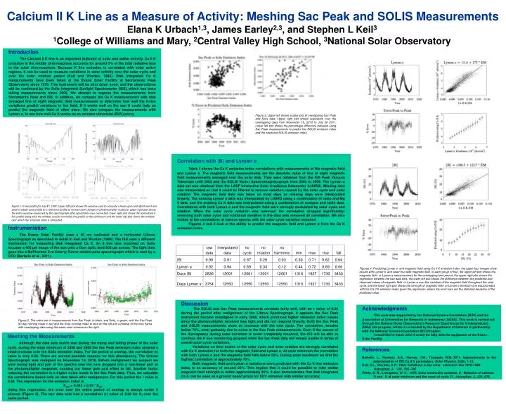
1. Calcium II K Line as a Measure of Activity: Meshing Sac Peak and SOLIS Measurements Elana K Urbach1,3, James Earley2,3, and Stephen L Keil3 1College of Williams and Mary, 2Central Valley High School, 3National Solar Observatory Introduction The Calcium II K line is an important indicator of solar and stellar activity. Ca II K emission in the middle chromosphere accounts for around 5% of the total radiativeloss in the solar chromosphere. Because K line emission is correlated with solar active regions, it can be used to measure variations in solar activity over the solar cycle and over the solar rotation period (Keil and Worden, 1984). Disk integrated Ca K measurements have been taken at the Evans Solar Facility at Sacramento Peak Observatory since 1976. This instrument will be shut down soon, and the observations will be continued by the Solis Integrated Sunlight Spectrometer (ISS), which has been taking measurements since 2006. We attempt to regress the measurements from Sacramento Peak and ISS. In addition, we compare the Ca K measurements with disk averaged line of sight magnetic field measurements to determine how well the K-line variations predict variations in the field. If it works well on the sun it could help us predict the magnetic field of other stars. We also compare the measurements with Lyman α, to see how well Ca K works as an extreme ultraviolet (EUV) proxy. Figure 3. Upper left shows scatter plot of overlapping Sac Peak and Solis data. Upper right plot shows regression over the overlapping days from November 18, 2010 to July 28 2011. Lower left plot shows the percentage difference between using Sac Peak measurements to predict the SOLIS emission index and the observed SOLIS emission index. Photomultiplier Counts Photomultiplier Counts Correlation with |B| and Lyman α Table 1 shows the Ca K emission index correlations with measurements of the magnetic field and Lyman α. The magnetic field measurements are the absolute value of line of sight magnetic field measurements averaged over the solar disk. They were obtained from the Kitt Peak Vacuum Telescope until 2003 and the SOLIS Vector Spectromagnetograph from 2003 to 2009. The Lyman α data set was obtained from the LASP Interactive Solar Irradiance Datacenter (LISIRD). Missing data was interpolated so that it could be filtered to remove variation caused by the solar cycle and solar rotation. The magnetic field data was taken on most days so missing days were interpolated linearly. The missing Lyman α data was interpolated by LISIRD using a combination of radio and Mg II data, and the missing Ca K data was interpolated using a combination of sunspot and radio data. Correlations with both Lyman α and the magnetic field were strongly modulated by solar cycle and rotation. When the solar cycle variation was removed, the correlation dropped significantly: removing both solar cycle and rotational variation in the data sets removed all correlation. We also looked at the correlations at various epochs with the solar cycle variation removed. Figures 4 and 5 look at the ability to predict the magnetic field and Lyman α from the Ca K emission index. Pixels Pixels Figure 1:K line profile for July 4th, 1991. Upper left plot shows the window used to compute a linear gain and offset which are used to adjust each profile to a reference profile to remove slow changes in photomultiplier response, upper right plot shows the entire window measured by the spectrograph after apodization by a cosine bell, lower right plot shows the normalized K line profile along with the window used to normalize the profile to the continuum and the lower left plot shows the window over which the emission index is computed. Instrumentation The Evans Solar Facility uses a 30 cm coelostat and a horizontal Littrow Spectrograph as described in detail in Keil and Worden (1984). The ISS uses a different mechanism for measuring disk integrated Ca K. An 8 mm lens mounted on Solis focuses a 400 µm image of the sun onto a fiber optic feed 600 µm across. The light then goes into a McPherson 2-m Czerny-Turner double-pass spectrograph which is read by a CCD (Bertello et al., 2011). Figures 4:Predicting Lyman α and magnetic field using Ca II K emission index: the upper four images show results with Lyman α and lower four with magnetic field. In each group of four, the upper left plot shows the magnetic field or Lyman α measurements for the overlapping time period, the upper right plot shows the regression between the two data sets, the lower left plot shows the difference between the predicted and observed values of magnetic field or Lyman α over the variation of the magnetic field throughout the solar cycle, and the lower right plot shows the strength of magnetic field or Lyman α emission one would predict with the Ca II K emission index given the regression, where the error bars are the standard deviation of the predicted value. Discussion The SOLIS and Sac Peak measurements correlate fairly well, with an r value of 0.68 during the period after realignment of the Littrow Spectrograph. It appears the Sac Peak instrument became misaligned in early 2008, which produced higher emission index values since the photomultiplier received less light and did not respond linearly. Both the Sac Peak and SOLIS measurements show an increase with the new cycle. The correlation remains below 70%, most probably due to noise in the Sac Peak measurements. Even if the source of the discrepancy during solar minimum is never completely resolved, the ISS will be able to continue the K line monitoring program while the Sac Peak data will remain usable in terms of overall solar cycle variations. Variations on time scales of the solar cycle and solar rotation are strongly correlated with Ca K emission for both the magnetic field and Lyman α. At solar minimum the correlation with both Lyman α and the magnetic field falls below 50%. During solar maximum we find the highest correlation of approximately 70%. Both magnetic field and Lyman α variations were predicted with the Ca K line emission index to an accuracy of around 20%. This implies that it could be possible to infer stellar magnetic field strength to within approximately 20%. It also demonstrates that disk integrated Ca K can be used as a ground based proxy for EUV emission with similar accuracy. Acknowledgments This work was supported by the National Science Foundation (NSF) and the Association of Universities for Research in Astronomy (AURA). This work is carried out through the National Solar Observatory’s Research Experiences for Undergraduate (REU) site program, which is co-funded by the Department of Defense in partnership with the National Science Foundation REU Program. I would like to thank John Cornett for help with the equipment at the Evans Solar Facility. Figure 2. The entire set of measurements from Sac Peak, in black, and Solis, in green, with the Sac Peak 90 day running mean in red and the Solis running mean in blue on the left and a blowup of the time frame with overlapping data using the same color scheme on the right. Meshing the Measurements Although the data sets match well during the rising and falling phase of the solar cycle, during the solar minimum of 2008 and 2009 the Sac Peak emission index showed a small increase over the Solis emission index. For the period of overlap, the correlation (r) value is only 0.54. There are several possible reasons for this discrepancy. The Littrow Spectrograph was realigned on November 18, 2010. Before realignment we suspect we were losing light and part of the spectra near the core dropped into a non-linear part of the photomultiplier response, causing our linear gain and offset to fail. Another factor reducing the correlation is a higher noise levels in the Sac Peak data. Thus, we calculate the correlations based only on data taken after realignment. For this period the r value is 0.68. The regression for the emission index is KISS = 0.043 + 0.53 * KSP Using this regression, the error over the entire period of overlap is always under 5 percent (Figure 3). The two data sets had a correlation (r) value of 0.66 for K3 over the same period. References Bertello, L., Pevtsov, A.A., Harvey, J.W., Toussain, R.M.:2011, Improvements in the determination of ISS Ca II K parameters. Solar Physics. 3(20), 1-16. Keil, S.L., Worden, S.P.: 1984, Variations in the solar calcium K line 1976-1982. Astrophys. J. 276, 766 -781. White, O. R., Livingston, W. C.: 1978, Solar luminosity variation. II - Behavior of calcium H and K at solar minimum and the onset of cycle 21. Astrophys. J., 226, 679.