Download
1 / 33
330 likes | 341 Views
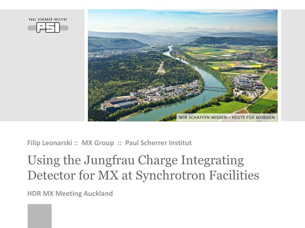
Filip Leonarski :: MX Group :: Paul Scherrer Institut. Using the Jungfrau Charge Integrating Detector for MX at Synchrotron Facilities. HDR MX Meeting Auckland. Presentation Plan. Jungfrau Detector Characteristics Jungfrau Pixel Output Data Conversion HDF5 Practicalities.

E N D
Filip Leonarski :: MX Group :: Paul Scherrer Institut Using the Jungfrau Charge Integrating Detector for MX at Synchrotron Facilities HDR MX Meeting Auckland
Presentation Plan • Jungfrau Detector Characteristics • Jungfrau Pixel Output • Data Conversion • HDF5 Practicalities
Jungfrau Detector JF4M at X06SA / SLS Dark current (pedestal) Leonarskiet al., Nat Methods, 15, 799-804 (2018) • Designed for SwissFEL, but with synchrotron applications in mind • Charge integrating • Shares EIGER design • Pixel size 75x75 μm • One ASIC = 256x256 pixels • One module = 4x2 ASICs = 1024x512 pixels • Adaptive gain • High dynamic range • Single photon sensitivity
Jungfrau for Macromolecular Crystallography Leonarskiet al., Nat Methods, 15, 799-804 (2018) • Photon counting detectors are state-of-the-art for conventional MX • Jungfrau can improve results for particular areas: • Low energy MX (≤ 6 keV) • Threshold limitations in HPC • High dose-rate experiments • Count-rate limitation in HPC • Jungfrau is necessary for sources with short, intense pulses: • XFEL • Pink beam and chopper
Jungfrau for Macromolecular Crystallography Leonarskiet al., Nat Methods, 15, 799-804 (2018) • Photon counting detectors are state-of-the-art for conventional MX • Jungfrau can improve results for particular areas: • Low energy MX (≤ 6 keV) • Threshold limitations in HPC • High dose-rate experiments • Count-rate limitation in HPC • Jungfrau is necessary for sources with short, intense pulses: • XFEL • Pink beam and chopper
High Dose-rate Strategy Casanaset al., Acta Cryst, D72, 1036-1048 (2016) Photon counting detectors introduce imprecisions for pixels with high photon rate due to pile-up effect In practice with a photon counting detector, for a well diffracting crystal one needs to attenuate beam and slow down measurement to get the best performance (see Casanaset al., Acta Cryst, D72, 2016)
High Dose-rate Strategy Leonarskiet al., Nat Methods, 15, 799-804 (2018) Photon counting detectors introduce imprecisions for pixels with high photon rate due to pile-up effect In practice with a photon counting detector, for a well diffracting crystal one needs to attenuate beam and slow down measurement to get the best performance (see Casanaset al., Acta Cryst, D72, 2016) Jungfrau has no such limitation
High Dose-rate Strategy Leonarskiet al., Nat Methods, 15, 799-804 (2018) • Photon counting detectors introduce imprecisions for pixels with high photon rate due to pile-up effect • In practice with a photon counting detector, for a well diffracting crystal one needs to attenuate beam and slow down measurement to get the best performance (see Casanaset al., Acta Cryst, D72, 2016) • Jungfrau has no such limitation • Jungfrau + DLSR, better magnets and novel sample delivery methods: • Higher beamline throughput • Fragment screening methods (<10s/xtal) • Routinely 100% flux and 50-100o/s with good data
Jungfrau Pixel Output Pixel output in JF: 0101010111110011 0001010111110011 Gain: 00:G0 01:G1 11:G2 0001010111110011 ADC value:
Jungfrau Pixel Output Pixel output in JF: 0101010111110011 0001010111110011 Gain: 00:G0 01:G1 11:G2 0001010111110011 ADC value: = Photon number:
Jungfrau Pixel Output Pixel output in JF: 0101010111110011 0001010111110011 Gain: 00:G0 01:G1 11:G2 0001010111110011 ADC value: Dedicated dark run = Gain and pedestal factors are specific for pixel and gain setting Photon number: Prior calibration
Jungfrau Pixel Output Pixel output in JF: 0101010111110011 0001010111110011 Gain: 00:G0 01:G1 11:G2 0001010111110011 ADC value: = G0 pedestal varies with time and needs to be tracked Photon number:
Jungfrau Pixel Output Photons Detector restarted after pedestal data taking Pixel output in JF: 0101010111110011 Pedestal 0001010111110011 Gain: 00:G0 01:G1 11:G2 0001010111110011 ADC value: Pedestal increases with longer integration time and higher temperature (higher framerate is always better) Redford et al., JINST, 13, C11006 = Photon number:
Jungfrau Pixel Output Pixel output in JF: 0101010111110011 0001010111110011 Gain: 00:G0 01:G1 11:G2 0001010111110011 ADC value: Pedestal increases with longer integration time and higher temperature (higher framerate is always better) = Photon number:
Jungfrau Pixel Output Pixel output in JF: 0101010111110011 0001010111110011 Gain: 00:G0 01:G1 11:G2 0001010111110011 ADC value: • Floating point number • Negative counts possible (not handled by data processing software at the moment) • Fractional counts relevant (charge sharing) = Photon number:
Jungfrau Data Conversion • Currently, both raw data and converted data are stored • Raw data do not compress very well • Raw data are necessary for detector development • Raw data will most likely not benefit end user • Converted data are already of very good quality • For user operation only converted data should be kept and these will be very similar to data produced by EIGER • Currently we imitate EIGER very well (REST interface and HDF5)
Jungfrau Data Conversion Challenge • Fast operation is necessary for good detector performance • 1.1 kHz at the moment, 2.4 kHz next year • Pedestal values depend on temperature of the sensor and should be collected within a short delay from the experiment • One needs to convert ADUs to photons to add frames together: • 5916 ADU in G0 + 300 ADU in G1 = ? • Since conversion factors are specific for pixel, gain setting and detector conditions, hardware lookup tables cannot be used for that purpose • One needs a floating point unit: CPU, GPU or Field Programmable Gate Array (FPGA)
Jungfrau Data Conversion Challenge • Data flow for 4M detector: • 4,194,304 pixels x 16-bit = 8 MB • 8 MB * 1.136 kHz = 9 GB/s ( 72 Gbit/s or 8x10 GbE links) • 8 MB * 2.400 kHz = 19 GB/s (153 Gbit/s or 16x10 GbE links) • Raw data need to be received by a computer, before calculations can be performed on CPU/GPU • There is no space for transmission control protocol (TCP) overhead, so if frames are not received, they are lost • x86-64/Linux machines are not designed for real time applications • With HPE DL580 Gen10 (4x12C Intel Xeon 6148 + 1.5 TB of RAM) we can handle both data receiving and data conversion for 4M @ 1.1 kHz, but not simultaneously
Converter Architecture Module: 1024x512 Module coordinates Module: 1030x514 4M detector coordinates Module 0 Pedestal and gain Summation Geometry (gaps, multipixels) Image 1 Image 2 Module 7 Frames • Input data • Placed in 4 RAM disks (2 modules per RAM disk) • Separate files per module • Modules (even pixels) are independent for conversion purpose • Output data • Compressed HDF5 file with NeXuS (Dectris flavor) metadata for Albula/Neggia • Compression operates on full images, so needs to combine all modules in one place • It is currently impossible to have separate HDF5 files for each region
Jungfrau Data Conversion Challenge 12 core Intel Xeon Skylake 12 core Intel Xeon Skylake 12 core Intel Xeon Skylake 12 core Intel Xeon Skylake JF detector module 1.1 GB/s JF detector module 1.1 GB/s JF detector module 1.1 GB/s JF detector module 1.1 GB/s Images in JF4M coordinates 2-port 10 GbE card 2.2 GB/s 2-port 10 GbE card 2.2 GB/s 2-port 10 GbE card 2.2 GB/s 2-port 10 GbE card 2.2 GB/s NUMA aware RAMdisk Tot. 1.5 TB NUMA aware RAMdisk Tot. 1.5 TB NUMA aware RAMdisk Tot. 1.5 TB NUMA aware RAMdisk Tot. 1.5 TB Image conversion Image conversion Image conversion Image conversion JF detector module 1.1 GB/s JF detector module 1.1 GB/s JF detector module 1.1 GB/s JF detector module 1.1 GB/s
Jungfrau Data Conversion Challenge 12 core Intel Xeon Skylake 12 core Intel Xeon Skylake 12 core Intel Xeon Skylake 12 core Intel Xeon Skylake 12 core Intel Xeon Skylake JF detector module 1.1 GB/s JF detector module 1.1 GB/s JF detector module 1.1 GB/s JF detector module 1.1 GB/s JF detector module 1.1 GB/s 2-port 10 GbE card 2.2 GB/s 2-port 10 GbE card 2.2 GB/s 2-port 10 GbE card 2.2 GB/s 2-port 10 GbE card 2.2 GB/s 2-port 10 GbE card 2.2 GB/s NUMA aware RAMdisk 120 GB/s NUMA aware RAMdisk Tot. 1.5 TB NUMA aware RAMdisk Tot. 1.5 TB NUMA aware RAMdisk Tot. 1.5 TB NUMA aware RAMdisk Tot. 1.5 TB Image conversion Image conversion Image conversion Image conversion Image conversion JF detector module 1.1 GB/s JF detector module 1.1 GB/s JF detector module 1.1 GB/s JF detector module 1.1 GB/s JF detector module 1.1 GB/s
Total Performance • 32 converter threads (4 per module) • 16 writer threads • Single instruction multiple data optimizations (AVX-512 for Intel Xeon) • Protein crystal • 87290 frames (+3000 pedestal) • 3 s pedestal • ~76 s of data collection * - throughput based on input frame size only, i.e. 8 MB/frame time • Execution time includes all steps, from reading raw data to writing final HDF5 • Compression time is non-deterministic (depends on data entropy)
Core Utilization – Intel VTune Summation of 10 Summation of 1
Floating-Point Unit Load – Intel VTune Summation of 10 Summation of 1
Microarchitecture Utilization – Intel VTune Summation of 10 Summation of 1
Data Challenge Conclusions • Data receiving needs to be offloaded by network boards with FPGA chips, writing raw frames directly to memory without CPU/kernel involvement • Jungfrau 4M @ 1.1 kHz possible in real time • Jungfrau 10M @ 2.4 kHz – most likely impossible with a single PC • Computational complexity is very limited (3% of FPU utilization) • Memory transfers are the limiting factor • GPU is not easy answer, as PCI Express is a bottleneck • More severe problem for multi-PC system • Virtual datasets (separate data files for 2D regions) could help a lot • Architectures optimized for higher data throughput are needed (IBM POWER) or hybrid architectures FPGA+Xeon / FPGA+ARM
Data Challenge Conclusions High data rate challenge of Jungfrau is driven by operational reasons, mainly related to dark current, however solving the challenge will benefit MX scientific goals High dose-rate strategy requires fast framerate detectors to achieve reasonable phi-slicing – to get 0.10o/image one needs: 1.0 kHz for full area of the detector at 100o/s rotation speed 2.0 kHz for full area of the detector at 200o/s rotation speed 2.4 kHz for full area of the detector at 360o/s rotation speed 0.15o/image Data processing will need to follow and we already need to think on GPU/FPGA/TPU/? implementations, due to Moore’s Law limitations
HDF5 Format Practicalities • Virtual datasets would allow data from separate modules could be compressed and written independently, without a need to gather all data before • Parallelization is highly limited by lack of fully thread-safe libhdf5 • Signed integer for photon counts: pedestal distribution can result in negative counts • Amplification factor (gain) in metadata: Jungfrau can report partial (half, quarter) photons in case of charge sharing, fixed-point format (2, 4, 8 or 16 counts per photon) would be better and easier than floating point storage • No count rate correction and per pixel saturation level • Compression • Bitshuffle: AVX-512 instructions library, FPGA implementation should be trivial • Hardware accelerated compression (IBM POWER9, NVIDIA GPUs) • Sparse data format: assuming 0 or 1 photons per pixel/frame Jungfrau allows to calculate energy and position with precision higher than one pixel for each photon • Metadata: For XFEL applications each frame is associated with metadata – saving these results in a very poor performance
Wir schaffen Wissen – heute für morgen Mythanksgoto • PSI Detector Group • Sophie Redford • Aldo Mozzanica • Bernd Schmitt • PSI MX Group • ZacPanepucci • Meitian Wang • PSI IT Group • Leonardo Sala • Dmitry Ozerov • Heiner Billich • Derek Feichtinger • Photon Factory KEK • NaohiroMatsugaki • Yusuke Yamada • Dectris • Stefan Brandstetter • Andreas Förster