Mapping the Baltic Sea Basin

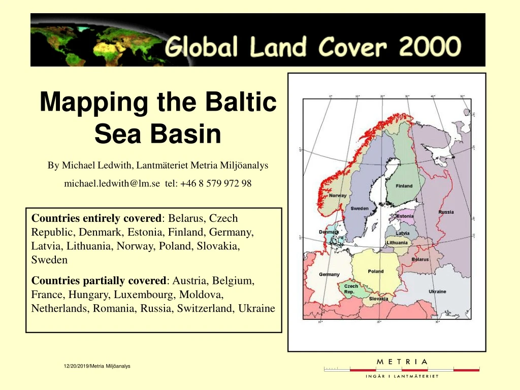
1. Mapping the Baltic Sea Basin By Michael Ledwith, Lantmäteriet Metria Miljöanalys michael.ledwith@lm.se tel: +46 8 579 972 98 Countries entirely covered: Belarus, Czech Republic, Denmark, Estonia, Finland, Germany, Latvia, Lithuania, Norway, Poland, Slovakia, Sweden Countries partially covered: Austria, Belgium, France, Hungary, Luxembourg, Moldova, Netherlands, Romania, Russia, Switzerland, Ukraine

2. Classification of the Baltic Sea Basin was carried out using low resolution (2250 km swath width) images acquired by the Vegetation instrument on-board the SPOT satellite. Four spectral bands: Blue: 0.43 - 0.47 m Red: 0.61 - 0.68 m Near Infrared (NIR): 0.78 - 0.89 m Mid Infrared (MIR): 1.58 - 1.75 m Additional information (based on ground reflectance) accompanying the radiometric data includes: NDVI / Status Map / Viewing Zenith Angle / Solar Zenith Angle / Viewing Azimuth Angle / Solar Azimuth Angle / Synthesis Time Grid SPOT Vegetation Images

3. North and south of ~32º, the VGT sensor acquires more than one image per day due to it’s wide swath. The daily synthesis composites (S-1) are computed from the different passes of one day for each location. In the high latitudes, each pass reflects different viewing and solar angles. The ten-day synthesis is computed from all of the passes for each location acquired during the ten-day period. The synthesis is created using the following criteria: SPOT VGT S-1 and S-10 Composites • the pixel does not correspond to a blind or interpreted pixel, • the pixel is not flagged as cloudy in the status map, • the pixel has the highest TOA NDVI compared with other pixels at the same location.

4. • conversion of S-10 file format from HDF to generic binary, • importing band data into image processing software (e.g. Erdas), • adding projection information (Platt-Carre) to images, • creating a five-band stacked image of the four radiometric bands and NDVI, • masking out the blind and aberrant MIR pixels, • masking out the compositing shadow effect at the land borders, • masking out clouds, • masking out water, • masking out snow and ice. Pre-processing SPOT VGT data

5. Blind and aberrant MIR pixels • • The MIR sensor consists of 6 bricks of 300 detectors in line. At every brick junction there is a blind detector. Therefore, inbetween the 6 bricks there are 5 blind spots. • • The MIR detectors are sensitive to proton fluxes coming from the sun. When a proton hits a detector, it is disturbed or destroyed, depending on the power of the proton or the number of the previous chocks it has received. On average, one detector is blind or aberrant per month. • • Prior to 17 May 2001 when CTIV initiated a more rigorous algorithm to remove these pixels, several northeast-southwest stripes are present on all of the images.

6. Edge Detection applied to image Resultant mask of blind/ aberrant MIR pixels Removing the blind and aberrant MIR pixels • A simple edge detection filter oriented northeast-southwest was applied to the MIR band. A minimum (black) and maximum (white) threshold was then applied to the image. This was very effective in removing the unwanted noise from the image.

7. Compositing Shadow Effect • For the calculation of synthesis images, the compositing method utilizes selection of maximum NDVI as the main rule. Over land, cloudy pixels generally have a lower NDVI than pixels where the land surface is visible. As a consequence, the compositing method tends to reject cloudy pixels over land in favor of non-cloudy pixels. However, over water where the cloud pixel has a higher NDVI value the situation is reversed and the cloud pixel is chosen over the water pixel. • A land-water mask is applied to the synthesis images which is slightly over-dimensioned for the land masses in order to cope with local inaccuracies. As a result, a roughly four pixel wide border of water/cloud pixels surrounds the land masses. Additionally, all water bodies (i.e. lakes, large rivers) show this effect as well.

8. Removing the compositing shadow effect Before • Simple masking of the compositing shadows based on spectral signatures could not be applied to the image due to the presence of similarly valued pixels over the mountainous regions of Norway, Sweden and southern Germany (snow, ice, rock and/or bare soil). • Several techniques were used with varying degrees of success to remove the effect including: • • unsupervised classification using 100 classes in order to find a “shadow” class, • • area specific region growing according to spectral properties using 8-directional neighborhoods and a Euclidean distance of between 20 and 250, • The final mask was constructed by clipping out 75 small areas along cloud free coastlines of S-1 images (2000-06-07 and 2000-09-12 to -21). In three cases, S-10 images from 2000-06-01, 2000-06-11 and 2000-09-21 were used. • These areas were processed using unsupervised classification (20 classes). The classes corresponding to compositing shadow were selected and joined in a composite mask. Clump (8-directions) and sieve processes were performed to remove snow/ice clusters and extraneous pixels. The final map used a sieve of 50 pixels initially and then a final sieve of 2 pixels. After

9. The SPOT VGT sensor has a linear array which greatly reduces the amount of distortion associated with off-nadir pixels - especially compared with scanning arrays such as AVHRR. However, at angles greater than approximately 50° distortion begins to effect the pixel size. Thus pixels which have been acquired at angles equal to or greater than 50° should be removed from the image prior to processing and classification. Using ancillary data which accompanies the radiometric data (i.e. viewing zenith angle file) a mask was created to remove distorted pixels. In most cases the removal of these data did not greatly affect the overall usability of the image. However, sometimes large swaths of data were removed and this greatly affected individual classifications. Removal of highly off-nadir pixels

10. Several different techniques were tested in order to determine the best method of accurately classifying the SPOT VGT S-10 images. For the most part, unsupervised classification on single S-10 composite images performed an adequate job at differentiating between the major types of land cover (i.e. forest, herbaceous, water, snow, sparse vegetation). Urban pixels are very difficult to classify using low resolution images and were identified using ancillary data. Due to several factors, the mountainous regions of Norway and Sweden proved to be an exception. Additionally, the make up of the forests of northern Sweden, Finland and eastern Russia - which contain perhaps thousands of lakes and bogs - makes it difficult to consistently classify these pixels accurately. Supervised classification using Maximum Likelihood, Mahalanobis Distance and Minimum Distance all failed to adequately classify western Scandinavia. Principal components analysis showed great potential in classification but due to time constraints this could not be further investigated. However, certain generalizations can be made relating to a PCA run on VGT radiometric data with 5 PC band output. PC1 - clearly differentiates between closed needle-leaf forest and other forms of landcover, PC2 - ideal band for identifying (and removing) water and snow pixels - particularly with respect to the water/cloud ring. Classification of S-10 images

11. Unsupervised Classification • The result of the unsupervised classification was a single band image consisting of clusters, or groupings, of areas in which the pixels show similar spectral signatures in most or all of the input bands. The results of an unsupervised classification, conducted on an S-10 composite image for 2000-09-21, are shown in to the right. The image is centered on the Polish city of Poznań, visible as a dark purple cluster. The large swaths of pink are agricultural lands where the crops have been harvested. The dark green areas are needle-leaf evergreen stands. The Bydgoszcz Canal and Noteć River are quite obvious as a light green linear feature, running east-west near the top of the image. Other agricultural areas, grasslands and deciduous forests are represented as a light green. The black speckles along the right side of the image are pixels that were masked out during the pre-processing of the image. • Results of unsupervised classification of four band VGT image with 40 classes as output, and a maximum of 15 iterations and a convergence threshold of 0.95.

12. Classification Algorithm • Essentially a matrix is created that cross tabulates the data in the reference image with the results from the unsupervised classification. From this matrix, data such as the majority pixel (the most commonly occurring pixel) and the percentage of pixels (fraction of majority) within a particular cluster can be easily obtained. • During the classification process, a pixel can match the criteria for labeling a pixel within several of the classification steps. That is, a pixel can be assigned to different land cover classes. However, all information produced in the different steps are merged together into a single land cover dataset in a predefined priority order (parallelpiping), thus the pixel is assigned to the land cover class to which it has the highest likelihood of belonging.

13. Comparing Majority and Percentage Cluster Images 1: 89% 2: 7% 3: 1% 1: Croplands 2: Pastures 3: Wetlands 1: 97% 2: 2% 3: 0% 1: Croplands 2: Pastures 3: N/A Within the majority image, a cluster in the first band contains a value corresponding to the most frequent class as compared to the reference data. Within the percentage image, a cluster in the first band contains a value corresponding to the percentage of the cluster that is occupied by the class as identified in the majority image. In MAJ 1 above, the cluster corresponds to 97% croplands per the reference data, while the MAJ2 cluster corresponds to 89% croplands (as well as 7% pastures).

14. Algorithm Results • A three-band majority image for 2000-09-21. Dark green areas are needle-leaf evergreen forests while lighter green pixels show agricultural areas and deciduous broadleaf trees (Helsinki, Finland). • A three-band percentage image for 2000-09-21. Light areas have a higher degree of agreement with the reference data (Helsinki, Finland).

15. ”Correctly” Classified Areas The image to the right shows the “correctly classified” pixels in the 2000-06-01 S-10 composite image centered over Copenhagen, Denmark. Gold pixels are agricultural lands while the dark green pixels are needle-leaf evergreen forests. The pixels that have been declared as correctly classified are removed from the satellite scenes (masked to a zero value) and a second unsupervised classification is performed.

16. Using PC Analyses • The image to the left shows the third principal component from an analysis done on the four radiometric bands of a S-10 composite image from 2000-09-21. This component is particularly well suited to differentiate between vegetation (light) and non-vegetation (dark). In addition, snow covered areas are visible as bright white regions - due to sensor saturation.

17. Final ”Correctly” Classified Pixel Image • Here is a mosaic of all the ”correctly” classified pixels for 2000-09-21 as acquired during the second stage of classification. Gold indicates agricultural areas, dark green represents needle-leaf evergreen and mixed forests, red areas are sparsely vegetated and light brown pixels are pastures.

18. Filling in the gaps • The above left image shows the open evergreen and mixed forests. The lower left image shows the sparsely vegetated areas, bare rock and snow covered areas. • The above right image shows the wetlands and lichen covered areas. The below right image shows the mosiac class of mixed forest and croplands. • For the majority of these images, the individual cluster was individually compared with the reference data in order to classify the cluster.

19. Assembling the final image • The final image was created piecewise by mosaicking the least specific (or important) information first and then adding layer upon layer of more specific information. This was done to assure that the classes that were more difficult to identify and thus acquired using different and more specific techniques wouldn’t become lost within the grosser classifications, e.g. pasture being included in the agriculture class. It also allowed urban pixels to be placed correctly even if an urban area was classified as forest (due to the presence of many trees and parks).