Download

1 / 37
370 likes | 375 Views
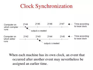
Clock Synchronization Chapter 9. TexPoint fonts used in EMF. Read the TexPoint manual before you delete this box.: A A A A A. Acoustic Detection (Shooter Detection). Sound travels much slower than radio signal (331 m/s) This allows for quite accurate distance estimation (cm)

E N D
Clock SynchronizationChapter 9 TexPoint fonts used in EMF. Read the TexPoint manual before you delete this box.: AAAAA
Acoustic Detection (Shooter Detection) • Sound travels much slower than radio signal (331 m/s) • This allows for quite accurate distance estimation (cm) • Main challenge is to deal with reflections and multiple events
Rating • Area maturity • Practical importance • Theoretical importance First steps Text book No apps Mission critical Not really Must have
Overview • Motivation • Clock Sources • Reference-Broadcast Synchronization (RBS) • Time-sync Protocol for Sensor Networks (TPSN) • Gradient Clock Synchronization
Motivation • Synchronizing time is essential for many applications • Coordination of wake-up and sleeping times (energy efficiency) • TDMA schedules • Ordering of collected sensor data/events • Co-operation of multiple sensor nodes • Estimation of position information (e.g. shooter detection) • Goals of clock synchronization • Compensate offset* between clocks • Compensate drift* between clocks • *terms are explained on following slides
Properties of Clock Synchronization Algorithms • External versus internal synchronization • External sync: Nodes synchronize with an external clock source (UTC) • Internal sync: Nodes synchronize to a common time • to a leader, to an averaged time, or to anything else • One-shot versus continuous synchronization • Periodic synchronization required to compensate clock drift • A-priori versus a-posteriori • A-posteriori clock synchronization triggered by an event • Global versus local synchronization (explained later) • Accuracy versus convergence time, Byzantine nodes, …
Clock Sources • Radio Clock Signal: • Clock signal from a reference source (atomic clock) is transmitted over a long wave radio signal • DCF77 station near Frankfurt, Germany transmits at 77.5 kHz with a transmission range of up to 2000 km • Accuracy limited by the distance to the sender, Frankfurt-Zurich is about 1ms. • Special antenna/receiver hardware required • Global Positioning System (GPS): • Satellites continuously transmit own position and time code • Line of sight between satellite and receiver required • Special antenna/receiver hardware required
Clock Devices in Sensor Nodes • Structure • External oscillator with a nominal frequency (e.g. 32 kHz) • Counter register which is incremented with oscillator pulses • Works also when CPU is in sleep state • Accuracy • Clock drift: random deviation from the nominal rate dependent on power supply, temperature, etc. • E.g. TinyNodes have a maximum drift of 30-50 ppm at room temperature This is a drift of up to 50 μs per second or 0.18s per hour Oscillator
Time accor- t t B ding to B 2 3 Answer Request from A from B t Time accor- t A ding to A 1 4 Sender/Receiver Synchronization • Round-Trip Time (RTT) based synchronization • Receiver synchronizes to the sender‘s clock • Propagation delay and clock offset can be calculated
Disturbing Influences on Packet Latency • Influences • Sending Time S (up to 100ms) • Medium Access Time A (up to 500ms) • Transmission Time T (tens of milliseconds, depending on size) • Propagation Time PA,B (microseconds, depending on distance) • Reception Time R (up to 100ms) • Asymmetric packet delays due to non-determinism • Solution: timestamp packets at MAC Layer S T A Timestamp TA R PA,B Timestamp TB Critical path
Some Details • Different radio chips use different paradigms: • Left is a CC1000 radio chip which generates an interrupt with each byte. • Right is a CC2420 radio chip that generates a single interrupt for the packet after the start frame delimiter is received. • In sensor networks propagationcan be ignored (<1¹s for 300m). • Still there is quite some variancein transmission delay because oflatencies in interrupt handling (picture right).
General Framework • The clock synchronization framework must provide the abstraction of a correct logical time to the application. This logical time is based on the (inaccurate) hardware clock, and calibrated by exchanging messages with other nodes in the network.
= + + + + t t S A P R 2 1 S S S , A A = + + + + t t S A P R 3 1 S S S , B B q = - = - + - t t ( P P ) ( R R ) 2 3 S , A S , B A B Reference-Broadcast Synchronization (RBS) • A sender synchronizes a set of receivers with one another • Point of reference: beacon’s arrival time A S B • Only sensitive to the difference in propagation and reception time • Time stamping at the interrupt time when a beacon is received • After a beacon is sent, all receivers exchange their reception times to calculate their clock offset • Post-synchronization possible • E.g., least-square linear regression to tackle clock drifts • Multi-hop?
0 1 1 1 2 2 2 2 Time-sync Protocol for Sensor Networks (TPSN) • Traditional sender-receiver synchronization (RTT-based) • Initialization phase: Breadth-first-search flooding • Root node at level 0 sends out a level discovery packet • Receiving nodes which have not yet an assigned level set their levelto +1 and start a random timer • After the timer is expired, a new level discovery packet will be sent • When a new node is deployed, it sends out a level request packet after a random timeout • Why this random timer?
Time-sync Protocol for Sensor Networks (TPSN) • Synchronization phase • Root node issues a time sync packet which triggers a random timer at all level 1 nodes • After the timer is expired, the node asks its parent for synchronization using a synchronization pulse • The parent node answers with an acknowledgement • Thus, the requesting node knows the round trip time and can calculate its clock offset • Child nodes receiving a synchronization pulse also start a random timer themselves to trigger their own synchronization 0 Time Sync 1 B ACK Sync pulse 1 2 A 2 2
= + + + + t t S A P R 0 2 1 A A A , B B = + + + + t t S A P R 1 B 4 3 B B B , A A - + - + - + - ( S S ) ( A A ) ( P P ) ( R R ) 1 2 q = A B A B A , B B , A B A 2 A 2 2 Time-sync Protocol for Sensor Networks (TPSN) • Time stamping packets at the MAC layer • In contrast to RBS, the signal propagation time might be negligible • Authors claim that it is “about two times” better than RBS • Again, clock drifts are taken into account using periodical synchronization messages • Problem: What happens in a non-tree topology (e.g. grid)? • Two neighbors may have bad synchronization?
Flooding Time Synchronization Protocol (FTSP) • Each node maintains both a local and a global time • Global time is synchronized to the local time of a reference node • Node with the smallest id is elected as the reference node • Reference time is flooded through the network periodically • Timestamping at the MAC Layer is used to compensate for deterministic message delays • Compensation for clock drift between synchronization messages using a linear regression table reference node 0 4 5 1 7 6 3 2
From single-hop to multi-hop • Many protocols don’t even handle single-hop clock synchronization well. On the left figures we see the absolute synchronization errors of TPSN and RBS, respectively. The figure on the right presents a single-hop synchronization protocol minimizing systematic errors. • Even perfectly symmetric errors will sum up over multiple hops. • In a chain of n nodes with a standard deviation ¾ on each hop, the expected error between head and tail of the chain is in the order of ¾√n.
Best tree for tree-based clock synchronization? • Finding a good tree for clock synchronization is a tough problem • Spanning tree with small (maximum or average) stretch. • Example: Grid network, with n = m2nodes. • No matter what tree you use, the maximumstretch of the spanning tree will always beat least m (just try on the grid figure right…) • In general, finding the minimum maxstretch spanning tree is a hard problem, however approximation algorithms exist [Emek, Peleg, 2004].
Local/Gradient Clock Synchronization • Global property: Minimize clock skew between any two nodes • Local (“gradient”) property: Small clock skew between two nodes if the distance between the nodes is small. • Clock should not be allowed to jump backwards • You don’t want new events to be registered earlier than older events. • Example: Root node 0 1 1 Small clock skew 1 2 2 2 3 3 3 4 4 Large clock skew
Trivial Solution: Let t = 0 at all nodes and times • Global property: Minimize clock skew between any two nodes • Local (gradient) property: Small clock skew between two nodes if the distance between the nodes is small. • Clock should not be allowed to jump backwards • To prevent trivial solution, we need a fourth constraint: • Clock should always to move forward. • Sometimes faster, sometimes slower is OK. • But there should be a minimum and a maximum speed.
0 1 2 3 0 1 2 3 0 1 2 3 0 1 2 3 Theoretical Bounds for Clock Synchronization • Network Model: • Each node i has a local clock Li(t) • Network with n nodes, diameter D. • Reliable point-to-point communication with minimal delay µ • Jitter ε is the uncertainty in message delay • Two neighboring nodes u, v cannot distinguish whether message is faster from u to v and slower from v to u, or vice versa. Hence clocks of neighboring nodes can be up to off. • Hence, two nodes at distance D may have clocks which are D off. • This can be achieved by a simple flooding algorithm: Whenever a node receives a new minimum value, it sets its clock to the new value and forwards its new clock value to all its neighbors. v v µ + µ µ µ + u u
Local/Gradient Clock Synchronization • Model • Each node has a hardware clock Hi(∙) with a clock rate hi(t) such that(1-²)t·hi(t) ·(1+²)t • The hardware clock of node i at time t is • Each node has a logical clock Li(∙) which increases at the rate of Hi(∙) • Employ a synchronization algorithm A to update the logical clock using the hardware clock and neighboring messages • The message transmission delay is in (0,1] Time is 152 Time is 142 Time is 140 Time is 150 ???
Synchronization Algorithms: Amax • Question: How to update the logical clock based on the messages from the neighbors? • Idea: Minimizing the skew to the fastest neighbor • Set the clock to the maximum clock value received from any neighbor(if greater than local clock value) • Poor local property: Fast propagation of the largest clock value could lead to a large skew between two neighboring nodes • First all messages take 1 time unit, then we have a fast message! New time is D+x skew D! New time is D+x Time is D+x Time is D+x Time is D+x … Old clock value:x Clock value:D+x Old clock value:D+x-1 Old clock value:x+1
Synchronization Algorithms: Amax’ • The problem of Amax is that the clock is always increased to the maximum value • Idea: Allow a constant slack γ between the maximum neighbor clock value and the own clock value • The algorithm Amax’ sets the local clock value Li(t) to → Worst-case clock skew between two neighboring nodes is still Θ(D) independent of the choice of γ! • How can we do better? • Adjust logical clock speeds to catch up with fastest node (i.e. no jump)? • Idea: Take the clock of all neighbors into account by choosing the average value?
Synchronization Algorithms: Aavg • Aavg sets the local clock to the average value of all neighbors: • Surprisingly, this algorithm is even worse! • We will now show that in a very natural execution of this algorithm, the clock skew becomes really large! Time is x+(n-1)2 Time is x+(n-2)2 Time is x+4 Time is x+1 n-1 n 2 1 … Clock value:x Clock value:x+(n-1)2 Clock value:x+(n-2)2 Clock value:x+1 skew 2n-3
Synchronization Algorithms: Aavg • Consider the following execution: • All i for i2 {1,…,n-1} are arbitrary values with i > 0. • The clock rates can be viewed as relative rates compared to the fastest node n. We will show: All messages arrive after 1 time unit! n n-1 1 … Clock rate:hn = 1 Clock rate:hn-1 = 1 - n-1 Clock rate:h1 = 1 - 1 Theorem: In the given execution, the largest skew between neighbors is 2n-3 2£(D). Hence, the global skew is £(D2).
Synchronization Algorithms: Aavg We first prove two lemmas: Lemma 1: In this execution it holds that 8t, 8i 2 {2,…,n}: Li(t) –Li-1(t) ≤ 2i – 3, independent of the choices of i > 0. Proof: Define Li(t) := Li(t) – Li(t-1). It holds that 8 t 8 i: Li(t) ≤ 1. L1(t) = L2(t-1), because node 1 has only one neighbor (node 2). Since L2(t) ≤ 1 for all t, we know that L2(t) – L1(t) ≤ 1 for all t. Assume now that it holds for 8t, 8j ≤ i: Lj(t) –Lj-1(t) ≤ 2j – 3. We prove a bound on the skew between node i and i+1: For t = 0 it is trivially true that Li+1(t) – Li(t) ≤ 2(i+1) – 3, since all clocks start with the same time.
Synchronization Algorithms: Aavg • Assume that it holds for all t’ ≤ t. For t+1 we have that • The first inequality holds because the logical clock value is always at least the average value of its neighbors. • The second inequality follows by induction. • The third and fourth inequalities hold because Li(t) ≤ 1. □
Synchronization Algorithms: Aavg Lemma 2: 8 i 2 {1,…,n}: limt !1Li(t) = 1. Proof: • Assume Ln-1(t) does not converge to 1. • Argument for simple case: 9 > 0 such that 8 t: Ln-1(t) ≤ 1 - . As Ln(t) is always 1, if there is such an , then limt !1Ln(t) - Ln-1(t) = 1, a contradiction to Lemma 1. • A bit more elaborate argument: Ln-1(t) = 1 only for some t, then there is an unbounded number of times t’ where Ln-1(t) < 1, which also implies that limt !1Ln(t) - Ln-1(t) = 1, again contradicting Lemma 1. Again, limt !1Ln-1(t) = 1. • Applying the same argument to the other nodes, it follows inductively that 8 i 2 {1,…,n}: limt !1Li(t) = 1. □
Synchronization Algorithms: Aavg Theorem: The skew between neighbors i and i-1converges to 2i-3. Proof: • We show that 8 i 2 {2,…,n}: limt !1 Li(t) – Li-1(t) = 2i – 3. • According to Lemma 2, it holds that limt !1 L2(t) – L1(t) = L1(t) = 1. • Assume by induction that 8 j ≤ i: limt !1 Lj(t) – Lj-1(t) = 2j – 3. • According to Lemmas 1 & 2, limt !1 Li+1(t) – Li(t) = Q for a value Q ≤ 2(i+1)-3. If (for the sake of contradiction) Q < 2(i+1)-3, then and thus limt !1Li(t) < 1, a contradiction to Lemma 2.□
Synchronization Algorithms: Abound • Idea: Minimize the skew to the slowest neighbor • Update the local clock to the maximum value of all neighbors as long as no neighboring node’s clock is more than B behind. • Gives the slowest node time to catch up • Problem: Chain of dependency • Node n-1 waits for node n-2, node n-2 waits for node n-3, …→ Chain of length Θ(n) = Θ(D) results in Θ(D) waiting time→Θ(D) skew! Time is x Time is x-B Time is x-2B n n-1 n-2 … Clock value:x Clock value:x - B Clock value:x - 2B
Synchronization Algorithms: Aroot • How long should we wait for a slower node to catch up? • Do it smarter: Set → skew is allowed to be→ waiting time is at most as well Waiting time Node withfast clock Skew Node withslow clock … Chain of length
Synchronization Algorithms: Aroot • When a message is received, execute the following steps: • This algorithm guarantees that the worst-case clock skew between neighbors is bounded by . max := Maximum clock value of all neighboring nodes min := Minimum clock value of all neighboring nodes if (max > own clock and min + > own clock own clock := min(max, min + ) inform all neighboring nodes about new clock value end if
Some Results • All natural/proposed clock synchronization algorithms seem to fail horribly, having at least square-root skew between neighbor nodes. • Indeed [Fan, Lynch, PODC 2004] show that when logical clocks need to obey minimum/maximum speed rules, the skew of two neighboring clocks can be up to (log D / log log D), where D is the diameter of the network. • Nice open problem…? Unfortunately not! In 2008 a O(log D) clock skew algorithm was presented at [Lenzen et al., FOCS 2008]. Also, the lower bound seems to be (log D)…
Theory vs. Practice • Can these theoretical findings be applied to practice? • Do the theoretical models represent reality? • Example: Experimental evaluation on a ring topology • Results: Synchronization error between Node 8 and Node 15 • Tree-based synchronization (FTSP, left) leads to a larger error than a simple gradient clock synchronization algorithm (right) Node 8 and Node 15 are leavesof two different subtrees
Open Problem • As listed on slide 9/6, clock synchronization has lots of parameters. Some of them (like local/gradient) clock synchronization have only started to be understood. • Local clock synchronization in combination with other parameters are not understood well, e.g. • accuracy vs. convergence • fault-tolerance in case some clocks are misbehaving [Byzantine] • clock synchronization in dynamic networks