Download
1 / 36
360 likes | 365 Views
This lecture provides a summary of Transactional Memory benefits, network topology examples, deadlock prevention, and packet/flit flow control in networks.

E N D
Lecture: Networks • Topics: TM wrap-up, networks
Summary of TM Benefits • As easy to program as coarse-grain locks • Performance similar to fine-grain locks • Avoids deadlock
Design Space • Data Versioning (when overflowing out of cache) • Eager: based on an undo log • Lazy: based on a write buffer • Conflict Detection • Optimistic detection: check for conflicts at commit time (proceed optimistically thru transaction) • Pessimistic detection: every read/write checks for conflicts (reduces work during commit)
TM Discussion • “Eager” optimizes the common case and does not waste energy when there’s a potential conflict • TM implementations require relatively low hardware support • Multiple commercial examples: Sun Rock, AMD ASF, IBM BG/Q, Intel Haswell
Network Topology Examples Hypercube Grid Torus
Routing • Deterministic routing: given the source and destination, there exists a unique route • Adaptive routing: a switch may alter the route in order to deal with unexpected events (faults, congestion) – more complexity in the router vs. potentially better performance • Example of deterministic routing: dimension order routing: send packet along first dimension until destination co-ord (in that dimension) is reached, then next dimension, etc.
Deadlock • Deadlock happens when there is a cycle of resource dependencies – a process holds on to a resource (A) and attempts to acquire another resource (B) – A is not relinquished until B is acquired
Deadlock Example 4-way switch Input ports Output ports Packets of message 1 Packets of message 2 Packets of message 3 Packets of message 4 Each message is attempting to make a left turn – it must acquire an output port, while still holding on to a series of input and output ports
Deadlock-Free Proofs • Number edges and show that all routes will traverse edges in increasing (or decreasing) order – therefore, it will be impossible to have cyclic dependencies • Example: k-ary 2-d array with dimension routing: first route along x-dimension, then along y 1 2 3 2 1 0 17 18 1 2 3 2 1 0 18 17 1 2 3 2 1 0 19 16 1 2 3 2 1 0
Breaking Deadlock • Consider the eight possible turns in a 2-d array (note that turns lead to cycles) • By preventing just two turns, cycles can be eliminated • Dimension-order routing disallows four turns • Helps avoid deadlock even in adaptive routing West-First North-Last Negative-First Can allow deadlocks
Packets/Flits • A message is broken into multiple packets (each packet has header information that allows the receiver to re-construct the original message) • A packet may itself be broken into flits – flits do not contain additional headers • Two packets can follow different paths to the destination Flits are always ordered and follow the same path • Such an architecture allows the use of a large packet size (low header overhead) and yet allows fine-grained resource allocation on a per-flit basis
Flow Control • The routing of a message requires allocation of various resources: the channel (or link), buffers, control state • Bufferless: flits are dropped if there is contention for a link, NACKs are sent back, and the original sender has to re-transmit the packet • Circuit switching: a request is first sent to reserve the channels, the request may be held at an intermediate router until the channel is available (hence, not truly bufferless), ACKs are sent back, and subsequent packets/flits are routed with little effort (good for bulk transfers)
Buffered Flow Control • A buffer between two channels decouples the resource allocation for each channel • Packet-buffer flow control: channels and buffers are allocated per packet • Store-and-forward • Cut-through • Wormhole routing: same as cut-through, but buffers in each router are allocated on a per-flit basis, not per-packet Time-Space diagrams 0 1 2 3 H B B B T H B B B T Channel H B B B T 0 1 2 3 H B B B T H B B B T Channel H B B B T 0 1 2 3 4 5 6 7 8 9 10 11 12 13 14 Cycle
Virtual Channels channel Buffers Buffers Flits do not carry headers. Once a packet starts going over a channel, another packet cannot cut in (else, the receiving buffer will confuse the flits of the two packets). If the packet is stalled, other packets can’t use the channel. With virtual channels, the flit can be received into one of N buffers. This allows N packets to be in transit over a given physical channel. The packet must carry an ID to indicate its virtual channel. Buffers Buffers Physical channel Buffers Buffers
Example • Wormhole: A is going from Node-1 to Node-4; B is going from Node-0 to Node-5 Node-0 B idle idle Node-1 A B Traffic Analogy: B is trying to make a left turn; A is trying to go straight; there is no left-only lane with wormhole, but there is one with VC Node-2 Node-3 Node-4 Node-5 (blocked, no free VCs/buffers) • Virtual channel: Node-0 B Node-1 A A A B Node-2 Node-3 Node-4 Node-5 (blocked, no free VCs/buffers)
Virtual Channel Flow Control • Incoming flits are placed in buffers • For this flit to jump to the next router, it must acquire three resources: • A free virtual channel on its intended hop • We know that a virtual channel is free when the tail flit goes through • Free buffer entries for that virtual channel • This is determined with credit or on/off management • A free cycle on the physical channel • Competition among the packets that share a physical channel
Buffer Management • Credit-based: keep track of the number of free buffers in the downstream node; the downstream node sends back signals to increment the count when a buffer is freed; need enough buffers to hide the round-trip latency • On/Off: the upstream node sends back a signal when its buffers are close to being full – reduces upstream signaling and counters, but can waste buffer space
Deadlock Avoidance with VCs • VCs provide another way to number the links such that a route always uses ascending link numbers 102 101 100 2 1 0 117 118 17 18 1 2 3 2 1 0 118 117 18 17 101 102 103 1 2 3 2 1 0 119 202 201 200 116 19 217 16 218 1 2 3 2 1 0 218 217 201 202 203 • Alternatively, use West-first routing on the 1st plane and cross over to the 2nd plane in case you need to go West again (the 2nd plane uses North-last, for example) 219 216
Router Functions • Crossbar, buffer, arbiter, VC state and allocation, buffer management, ALUs, control logic, routing • Typical on-chip network power breakdown: • 30% link • 30% buffers • 30% crossbar
Router Pipeline • Four typical stages: • RC routing computation: the head flit indicates the VC that it belongs to, the VC state is updated, the headers are examined and the next output channel is computed (note: this is done for all the head flits arriving on various input channels) • VA virtual-channel allocation: the head flits compete for the available virtual channels on their computed output channels • SA switch allocation: a flit competes for access to its output physical channel • ST switch traversal: the flit is transmitted on the output channel A head flit goes through all four stages, the other flits do nothing in the first two stages (this is an in-order pipeline and flits can not jump ahead), a tail flit also de-allocates the VC
Router Pipeline • Four typical stages: • RC routing computation: compute the output channel • VA virtual-channel allocation: allocate VC for the head flit • SA switch allocation: compete for output physical channel • ST switch traversal: transfer data on output physical channel STALL Cycle 1 2 3 4 5 6 7 Head flit Body flit 1 Body flit 2 Tail flit RC VA SA ST RC VA SA SA ST -- -- SA ST -- -- -- SA ST -- -- SA ST -- -- -- SA ST -- -- SA ST -- -- -- SA ST
Speculative Pipelines • Perform VA, SA, and ST in parallel (can cause collisions and re-tries) • Typically, VA is the critical path – can possibly perform SA and ST sequentially • Perform VA and SA in parallel • Note that SA only requires knowledge of the output physical channel, not the VC • If VA fails, the successfully allocated channel goes un-utilized Cycle 1 2 3 4 5 6 7 Head flit Body flit 1 Body flit 2 Tail flit RC VA SA ST RC VA SA ST -- SA ST SA ST -- SA ST SA ST -- SA ST SA ST • Router pipeline latency is a greater bottleneck when there is little contention • When there is little contention, speculation will likely work well! • Single stage pipeline?
Current Trends • Growing interest in eliminating the area/power overheads of router buffers; traffic levels are also relatively low, so virtual-channel buffered routed networks may be overkill • Option 1: use a bus for short distances (16 cores) and use a hierarchy of buses to travel long distances • Option 2: hot-potato or bufferless routing
Centralized Crossbar Switch P0 P1 P2 P3 P4 P5 P6 P7
Crossbar Properties • Assuming each node has one input and one output, a crossbar can provide maximum bandwidth: N messages can be sent as long as there are N unique sources and N unique destinations • Maximum overhead: WN2 internal switches, where W is data width and N is number of nodes • To reduce overhead, use smaller switches as building blocks – trade off overhead for lower effective bandwidth
Switch with Omega Network 000 P0 000 001 P1 001 010 P2 010 011 P3 011 100 P4 100 101 P5 101 110 P6 110 111 P7 111
Omega Network Properties • The switch complexity is now O(N log N) • Contention increases: P0 P5 and P1 P7 cannot happen concurrently (this was possible in a crossbar) • To deal with contention, can increase the number of levels (redundant paths) – by mirroring the network, we can route from P0 to P5 via N intermediate nodes, while increasing complexity by a factor of 2
Tree Network • Complexity is O(N) • Can yield low latencies when communicating with neighbors • Can build a fat tree by having multiple incoming and outgoing links P0 P1 P2 P3 P4 P5 P6 P7
Bisection Bandwidth • Split N nodes into two groups of N/2 nodes such that the bandwidth between these two groups is minimum: that is the bisection bandwidth • Why is it relevant: if traffic is completely random, the probability of a message going across the two halves is ½ – if all nodes send a message, the bisection bandwidth will have to be N/2 • The concept of bisection bandwidth confirms that the tree network is not suited for random traffic patterns, but for localized traffic patterns
Distributed Switches: Ring • Each node is connected to a 3x3 switch that routes messages between the node and its two neighbors • Effectively a repeated bus: multiple messages in transit • Disadvantage: bisection bandwidth of 2 and N/2 hops on average
Distributed Switch Options • Performance can be increased by throwing more hardware at the problem: fully-connected switches: every switch is connected to every other switch: N2wiring complexity, N2/4 bisection bandwidth • Most commercial designs adopt a point between the two extremes (ring and fully-connected): • Grid: each node connects with its N, E, W, S neighbors • Torus: connections wrap around • Hypercube: links between nodes whose binary names differ in a single bit
Topology Examples Hypercube Grid Torus
Topology Examples Hypercube Grid Torus
k-ary d-cube • Consider a k-ary d-cube: a d-dimension array with k elements in each dimension, there are links between elements that differ in one dimension by 1 (mod k) • Number of nodes N = kd Number of switches : Switch degree : Number of links : Pins per node : Avg. routing distance: Diameter : Bisection bandwidth : Switch complexity : Should we minimize or maximize dimension?
k-ary d-Cube • Consider a k-ary d-cube: a d-dimension array with k elements in each dimension, there are links between elements that differ in one dimension by 1 (mod k) • Number of nodes N = kd Number of switches : Switch degree : Number of links : Pins per node : N Avg. routing distance: Diameter : Bisection bandwidth : Switch complexity : d(k-1)/4 2d + 1 d(k-1)/2 Nd 2wkd-1 2wd (2d + 1)2 The switch degree, num links, pins per node, bisection bw for a hypercube are half of what is listed above (diam and avg routing distance are twice, switch complexity is ) because unlike the other cases, a hypercube does not have right and left neighbors. Should we minimize or maximize dimension? (d + 1)2
Title • Bullet