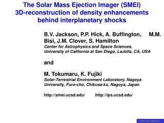
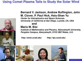
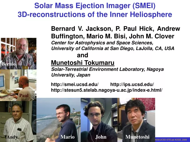
Bernard V. Jackson, P. Paul Hick, Andrew Buffington, Mario M. Bisi, John M. Clover

1. Bernard V. Jackson, P. Paul Hick, Andrew Buffington, Mario M. Bisi, John M. Clover Center for Astrophysics and Space Sciences, University of California at San Diego, LaJolla, CA, USA and Munetoshi Tokumaru Solar-Terrestrial Environment Laboratory, Nagoya University, Japan Bernie http://smei.ucsd.edu/ http://ips.ucsd.edu/ http://stesun5.stelab.nagoya-u.ac.jp/index-e.html/ Paul Andy Mario John Munetoshi Masayoshi

2. Introduction: SMEI and IPS remote-sensing data analyses Tomographic techniques used to determine Solar Wind 3D structure (examples). Comparisons at Mars

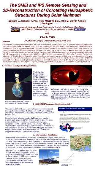
3. http://smei.ucsd.edu/ The Solar Mass Ejection Imager (SMEI) Mission (Solar Phys., 225, 177-207) B. V. Jackson, A. Buffington, P. P. Hick Center for Astrophysics and Space Sciences, University of California at San Diego, LaJolla, CA. R.C. Altrock, S. Figueroa, P.E. Holladay, J.C. Johnston, S.W. Kahler, J.B. Mozer, S. Price, R.R. Radick, R. Sagalyn, D. Sinclair Air Force Research Laboratory/Space Vehicles Directorate (AFRL/VS), Hanscom AFB, MA G.M. Simnett, C.J. Eyles, M.P. Cooke, S.J. Tappin School of Physics and Space Research, University of Birmingham, UK T. Kuchar, D. Mizuno, D.F.Webb ISR, Boston College, Newton Center, MA P.A. Anderson Boston University, Boston, MA S.L. Keil National Solar Observatory, Sunspot, NM R.E. Gold Johns Hopkins University/Applied Physics Laboratory, Laurel, MD N.R. Waltham Space Science Dept., Rutherford-Appleton Laboratory, Chilton, UK The SERP/STP Coriolis spacecraft at Vanden-berg prior to flight. The SMEI baffles are circled. The large NRL radiometer Windsat is on the top of the spacecraft.

4. Data!! Lots of Data!! Launch 6 January 2003 1 gigabyte/day; now ~3.5 terabytes  Sun C1 C2 C3 Sun | V Simultaneous images from the three SMEI cameras.

5. Frame Composite for Aitoff Map Blue = Cam3; Green= Cam2; Red = Cam1 D290; 17 October 2003

6. SMEI first light composite image Composite all-sky map 2 Feb 2003 from the three SMEI cameras.

7. Brightness fall-off with distance  A very tiny signal

8. 27-28 May 2003 CME events brightness time series for select sky sidereal locations With all contaminant signals eliminated, SMEI brightness is shown with a long-term temporal base removed. Data points are obtained on each SMEI orbit every 102-minutes, and the data here show a CME that has passed the Earth and is measured in situ. (1 S10 = 0.46 ± 0.02 ADU)

9. “Cleaned brightness” from the 28 May 2003 halo CMEat specific sidereal lines of sight over one 3-hour period

10. STELab IPS Heliospheric Analyses IPS line-of-sight response STELab IPS array near Fuji

11. Density Turbulence • Scintillation index, m, is a measure of level of turbulence • Normalized Scintillation index, g = m(R) / <m(R)> • g > 1  enhancement in Ne • g  1  ambient level of Ne • g < 1  rarefaction in Ne (CourtesyofP.K.Manoharan) A scintillation enhancement with respect to the ambient wind identifies the presence of a region of increased turbulence/density and a possible CME along the line-of-sight to the radio source.

12. STELab IPS Heliospheric Analyses The newest STELab IPS array at Toyokawa - photo 17 February 2007 (October IPS Workshop see: http://smei.ucsd.edu/ips_toyokawa.html)

13. Heliospheric C.A.T. Analyses 30º LOS Weighting 60º 90º The outward-flowing solar wind structure follows very specific physics as it moves outward from the Sun Thomson scattering

14. SMEI Heliospheric C.A.T. Analyses Line of sight “crossed” components on a reference surface. Projections on the reference surface are shown. These weighted components are inverted to provide the time-dependent tomographic reconstruction. A half-day difference

15. Heliospheric C.A.T. Analyses: example line-of-sight distribution for each sky location to form the source surface of the 3D reconstruction. STELab IPS 14 July 2000 13 July 2000

16. 27-28 May 2003 CME events SMEI density 3D reconstruction of the 28 May 2003 halo CME as viewed from 15º above the ecliptic plane about 30º east of the Sun-Earth line. Jackson et al., JGR. (2006) 111 (A4): A04S91 SMEI density (remote observer view) of the 28 May 2003 halo CME

17. 27-28 May 2003 CME events CME masses Jackson et al., JGR. (2006) 111 (A4): A04S91

18. 27-28 May 2003 CME event period Earth in situ comparison density SMEI proton density reconstruction of the May - June 2003 halo CME period compared with Wind over one Carrington rotation Jackson et al., JGR. (2006) 111 (A4): A04S91

19. SMEI Agreement with Sophisticated Modeling 27-28 May 2003 CME events HAF Model Comparison Brightness from the 28 May 2003 halo CME3D reconstruction (left) and HAF model (right). Jackson et al., JGR. (2006) 111 (A4): A04S91

20. 28 October 2003 CME Northeast-directed ejecta is more-nearly earth-directed. C2 image Southward ejecta Southward ejecta LASCO C2 CME image to 6 Rs. SMEI enhanced Sky Map image and animation to 110º elongation. Jackson et al., JGR. (2008) 113: A00A15 SMEI C.A.T. Analysis

21. Mass determination ~6.7  1016 g excess and 8.3  1016 g total for northward directed structure within the 10 e-cm-3 contour. SMEI 3D-reconstruction of the 28 October CME. The above structure has a mass of about 0.5  1016 g excess in the sky plane but ~ 2.0  1016 g excess at 60º (Vourlidas, private communication, 2004). SMEI C.A.T. Analysis

22. 28 October 2003 CME SMEI reconstructed density on 30`October at 03 UT 15 e- cm-3 to 30 e- cc-3. IPS 3D-reconstructed velocity at 03 UT viewed above 950 km s-1.

23. IPS and SMEI 3D reconstruction of the 28 October 2003 CME IPS g-level data reconstruction of density from data obtained between 22 UT 28 and 7 UT 29 October 2003. The reconstruction time is ~3 UT. Mass ~6  1016 g Reconstruction from SMEI data on 03 UT29 October 2003. Mass ~7  1016 g for the event northward portion

24. Recent higher-resolution SMEI PC 3D reconstructions show the CME sheath region as well as the central dense core 28 October 2003 CME higher-resolution analysis shock Ecliptic cut Meridional cut SMEI C.A.T. Analysis

25. 28 October 2003 CME higher-resolution analysis Ecliptic cuts Meridional cuts SMEI C.A.T. Analysis

26. Solar Wind Pressure derived from the MGS Magnetometer at Mars Crider et al., J. Geophys. Res. (2003) 108(A12): 1461

27. IPS 3D Reconstruction 28 May 2003 ‘Halo’ CME event sequence Density derived from IPS | Jackson et al., Solar Phys. (2007) 241: 385–396

28. IPS 3D-Reconstruction 20 May – 05 June 2003, (28 May ‘Halo’ CME) Pressure derived from IPS at Mars Solar Wind Pressure (ρ = 2 X 106 nV2) Jackson et al., Solar Phys. (2007) 241: 385–396

29. IPS 3D-Reconstruction 12 September – 26 September 2002 period Density Pressure (ρ = 2 X 106 nV2) Jackson et al., Solar Phys. (2007) 241: 385–396

30. IPS solar wind pressure 3D-reconstruction at Mars from 1999 - 2004 Time lags between ram pressure peaks (from a sample of 37 peaks). A positive shift indicates a lag in the IPS-derived pressure peak from that from MGS.

31. Summary: a) SMEI allows derivation of global densities including that from CMEs at high spatial and temporal resolution using Thomson-scattering brightness. b) IPS allows derivation of global velocity, and through conversion of g-level to density – global densities, at low resolution from STELab data, including for CMEs. c) These have been combined to compare with Mars Global Surveyor magnetometer data where solar wind pressure have been derived from 1999 – 2004. Still needed – IPS velocity data from more radio sources in order to provide better velocity resolutions in comparison with derived global densities.