Download

1 / 30
300 likes | 305 Views
Genome evolution. Lecture 5: Inference through sampling. Basic phylogenetics. Reminder: Inference. We assume the model (structure, parameters) is given, and denote it by q :. Alignment. Evolutionary rates. Tree. Ancestral Inference on a phylogenetic tree.

E N D
Genome evolution Lecture 5: Inference through sampling. Basic phylogenetics
Reminder: Inference We assume the model (structure, parameters) is given, and denote it by q: Alignment Evolutionary rates Tree Ancestral Inference on a phylogenetic tree The Total probability of the data s: Learning a model This is also called the likelihood L(q). Computing Pr(s) is the inference problem Easy! Given the total probability it is easy to compute: Exponential? Total probability of the data Posterior of hi given the data Marginalization over hi
With undirected cycles, the model is well defined but inference becomes hard 7 8 9 1 4 2 5 3 6 Two examples: What makes these examples difficult? We want to perform inference in an extended tree model q expressing context effects: 1 2 3 We want to perform inference on the tree structure itself! Each structure impose a probability on the observed data, so we can perform inference on the space of all possible tree structures, or tree structures + branch lengths q
More terminology: make sure you know how to define these: InferenceParameter learningLikelihoodTotal probability/Marginal probabilityExact inference/Approximate inference Sampling is the a natural way to do approximate inference Marginal Probability (integration over A sample) Marginal Probability (integration over all space)
7 8 9 4 5 6 Sampling from a BN How to sample from the CPD? Naively: If we could draw h,s’ according to the distribution Pr(h,s’) then: Pr(s) ~ (#samples with s)/(# samples) Forward sampling: use a topological order on the network. Select a node whose parents are already determined sample from its conditional distribution (all parents already determined!) Claim: Forward sampling is correct: 1 2 3
Why don’t we constraint the sampling to fit the evidence s? 1 2 3 7 8 9 4 5 6 Focus on the observations What is the sampling error? Two tasks: P(s) and P(f(h)|s), how to approach each/both? Naïve sampling is terribly inefficient, why? This can be done, but we no longer sample from P(h,s), and not from P(h|s) (why?)
7 8 9 Likelihood weighting • Likelihood weighting: • weight = 1 • use a topological order on the network. • Select a node whose parents are already determined • if the variable was not observed: sample from its conditional distribution • else: weight *= P(xi|paxi), and fix the observation • Store the sample x and its weight w[x] • Pr(h|s) = (total weights of samples with h) / (total weights) Weight=
Importance sampling Our estimator from M samples is: But it can be difficult or inefficient to sample from P. Assume we sample instead from Q, then: Prove it! Unnormalized Importance sampling: Claim: To minimize the variance, use a Q distribution is proportional to the target function:
Correctness of likelihood weighting: Importance sampling For the likelihood waiting algorithm, our proposal distribution Q is defined by fixing the evidence at the nodes in a set E and ignoring the CPDs of variable with evidence. We sample from Q just like forward sampling from a Bayesian network that eliminated all edges going into evidence nodes! Unnormalized Importance sampling with the likelihood weighting proposal distribution Q and any function on the hidden variables: Proposition: the likelihood weighting algorithm is correct (in the sense that it define an estimator with the correct expected value)
Sample: Normalized Importance sampling: Normalized Importance sampling When sampling from P(h|s) we don’t know P, so cannot compute w=P/Q We do know P(h,s)=P(h|s)P(s)=P(h|s)a=P’(h) So we will use sampling to estimate both terms: Using the likelihood weighting Q, we can compute posterior probabilities in one pass (no need to sample P(s) and P(h,s) separately):
Limitations of forward sampling observed Likelihood weighting is effective here: unobserved But not here:
Symmetric and reversible Markov processes Definition: we call a Markov process symmetric if its rate matrix is symmetric: What would a symmetric process converge to? Definition: A reversible Markov process is one for which: Time: t s i j j i qji Claim: A Markov process is reversible iff such that: pi pj If this holds, we say the process is in detailed balance and the p are its stationary distribution. qij Proof: Bayes law and the definition of reversibility
Q,t’ Q,t Q,t’ Q,t Q,t+t’ Reversibility qji Claim: A Markov process is reversible iff such that: pi pj If this holds, we say the process is in detailed balance. qij Proof: Bayes law and the definition of reversibility Claim: A Markov process is reversible iff we can write: where S is a symmetric matrix.
(Start from anywhere!) Markov Chain Monte Carlo (MCMC) We don’t know how to sample from P(h)=P(h|s) (or any complex distribution for that matter) The idea: think of P(h|s) as the stationary distribution of a Reversible Markov chain Find a process with transition probabilities for which: Process must be irreducible (you can reach from anywhere to anywhere with p>0) Then sample a trajectory Theorem: (C a counter)
The Metropolis(-Hastings) Algorithm Why reversible? Because detailed balance makes it easy to define the stationary distribution in terms of the transitions So how can we find appropriate transition probabilities? We want: Define a proposal distribution: And acceptance probability: F x y What is the big deal? we reduce the problem to computing ratios between P(x) and P(y)
Acceptance ratio for a BN To sample from: We will only have to compute: For example, if the proposal distribution changes only one variable hi what would be the ratio? We affected only the CPDs of hi and its children Definition: the minimal Markov blanket of a node in BN include its children, Parents and Children’s parents. To compute the ratio, we care only about the values of hi and its Markov Blanket
Gibbs sampling A very similar (in fact, special case of the metropolis algorithm): Start from any state h do { Chose a variable Hi Form ht+1 by sampling a new hi from } This is a reversible process with our target stationary distribution: Gibbs sampling is easy to implement for BNs:
A problematic space would be loosely connected: Examples for bad spaces Sampling in practice We sample while fixing the evidence. Starting from anywere but waiting some time before starting to collect data How much time until convergence to P? (Burn-in time) Mixing Sample Burn in Consecutive samples are still correlated! Should we sample only every n-steps?
Inferring/learning phylogenetic trees Distance based methods: computing pairwise distances and building a tree based only on those (how would you implement this?) More elaborated methods use a scoring scheme that take the whole tree into account, using Parsimony vs likelihood Likelihood methods: universal rate matrices (BLOSSOM62, PAM) Searching for the optimal tree (min parsimony or max likelihood) is NP hard Many search heuristics were developed, finding a high quality solution and repeating computation using partial dataset to test for the robustness of particular features (Bootstrap) Bayesian inference methods – assuming some prior on trees (e.g. uniform) and trying to sample trees from the probability space P(q|D). Using MCMC, we only need a proposal distribution that span all possible trees and a way to compute the likelihood ratio between two trees (polynomial for the simple tree model) From sampling we can extract any desirable parameter on the tree (number of time X,Y and Z are in the same clade)
Curated set of universal proteins Eliminating Lateral transfer Multiple alignment and removal of bad domains Maximum likelihood inference, with 4 classes of rate and a fixed matrix Bootstrap Validation Ciccarelli et al 2005
How much DNA? (Following M. Lynch) Viral particles in the oceans: 1030 times 104 bases = 1034 Global number of prokaryotic cells: 1030 times 3x106 bases = 1036 107 eukaryotic species (~1.6 million were characterized) One may assume that they each occupy the same biomass, For human, 6x10⁹ (population) times 6x10⁹ (genome) times 1013 (cells) = 1032 Assuming average eukaryotic genome size is 1% of the human, we have 1037bases
? ? RNA Based Genomes Ribosome Proteins Genetic Code DNA Based Genomes Membranes Diversity! Think ecology.. 3.4 – 3.8 BYA – fossils?? 3.2 BYA – good fossils 3 BYA – metanogenesis 2.8 BYA – photosynthesis .. .. 1.7-1.5 BYA – eukaryotes .. 0.55 BYA – camberian explosion 0.44 BYA – jawed vertebrates 0.4 – land plants 0.14 – flowering plants 0.10 - mammals
Eukaryotes Uniknots Biknots
Eukaryotes Uniknots – one flagela at some developmental stage Fungi Animals Animal parasites Amoebas Biknots – ancestrally two flagellas Green plants Red algea Ciliates, plasmoudium Brown algea More amobea Strange biology! A big bang phylogeny: speciations across a short time span? Ambiguity – and not much hope for really resolving it
Vertebrates Fossil based, large scale phylogeny Sequenced Genomes phylogeny
Primates 9% 1.2% 0.8% 3% 1.5% 0.5% 0.5% Gorilla Chimp Gibbon Baboon Human Macaque Marmoset Orangutan