Download
1 / 59
790 likes | 1.19k Views
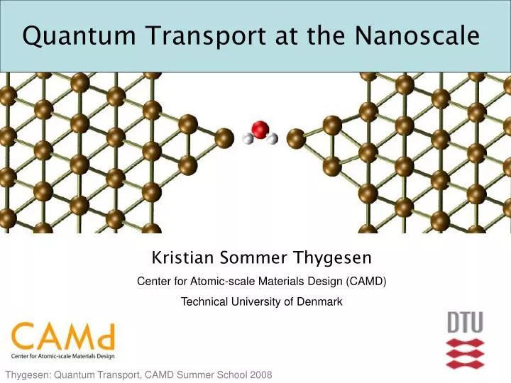
Quantum Transport at the Nanoscale. Kristian Sommer Thygesen Center for Atomic-scale Materials Design (CAMD) Technical University of Denmark. Moore’s Law. Gordon Moore (co-founder of Intel) 1965: The density of transistors on a chip will double every two years. Moore’s Law.

E N D
Quantum Transport at the Nanoscale Kristian Sommer Thygesen Center for Atomic-scale Materials Design (CAMD) Technical University of Denmark
Moore’s Law Gordon Moore (co-founder of Intel) 1965: The density of transistors on a chip will double every two years.
Moore’s Law Si-based transistor ~65 nm (2007). ENIAC computer, 1947 • Future challenges for semiconductor device technology: • Leak currents through gate oxide (improvement by high k materials) • Quantum confinement effects affect device functionality • Lithographic top-down printing of ever smaller features • Reliable doping of Si increasingly difficult
Molecular Electronics Bottom-up design of electronic components using single molecules. Advantages: (Potentially) cheap, truly nano-sized, flexibility in design and functionality. Challenges: Contacting molecules by electrodes, large-scale integration R. Stadler, M. Forshaw, and C. Joachim, Nanotechnology 14, 138 (2003) Example: A molecular switch: E. Lortscher et al., Small 2, 973 (2006)
Programme Part 1: Formalism and Methodology (40 min) Part 2: Coffee (10 min.) Part 3: Applications (40 min)
Part 1: Formalism and methodology • Definition of the problem • Two routes for solving the problem • Wave function method (scattering theory) • Green’s functions • Two limiting cases • Adiabatic approximation • Single resonant level model • Combining transport and DFT
Challenges: • Interacting electrons • Nonequilibrium • Interactions with molecular vibrations • Open boundary conditions Definition of the problem #1 Calculate the IVcurve! I
Definition of the problem #2 • Non-interacting electrons • Scattering free leads (perfect crystalline electrodes) • Electrons incident from left/right are in thermal equilibrium with left/right reservoirs. • Complete thermalization of electrons upon entering reservoir • No back scattering at lead-reservoir interface
Ballistic transport – single channel Ballistic: no scattering region. Single channel: one left/right moving state at each energy Steady state current: A ”ballistic channel” contributes to the conductance by 1G0. Note: This result is independent of the band structure!
Ballistic transport – many channels Each transverse mode defines a transport channel. M=2 Steady state current: M is number of modes within the bias window
Scattering In general, each incoming channel is scattered into a linear combination of several forward and backward moving channels. Landauer formula: |tnm(E)|2 : Probability that an electron with energy E injected in mode n is transmitted into mode m. Elastic transmission function: Linear response conductance:
Consider the following questions: • What is the conductance in the example shown above? • What happens as the constriction is further narrowed/opened? Slowly varying potentials Constricted quantum wire: Energy of transverse modes: Adiabatic ansatz: Adiabatic picture: As the electron moves along the x axis, energy is transferred from the longitudinal motion to the transverse mode.
Conductance quantization Numerical examples: Transmission in 2d quantum wires • For slowly varying constrictions, the conductance is quantized in units of G0. • Conductance quantization in quantum wires is a robust phenomenon. • Conductance steps are observable for kT << E’, where E’ is the spacing of transverse modes.
Conductance quantization in gold chains Chains of single metal atoms can be formed by breaking a nanocontact using e.g. an STM or mechanically controlled break junctions (MCBJ). Yanson et al. Phys. Rev. Lett. 95 256806 (2005) DFT molecular dynamics simulations by Sune Bahn.
Green’s functions – why? • More complex than density, less complex than wavefunction • Allow for systematic perturbation theory • Easy to handle in a computer • Straightforward to include interactions via self-energies, e.g. GW approximation • Straightforward to describe open boundary conditions • Seem rather abstract at first encounter • Do not always provide much physical insight
Green’s functions Green’s function (or resolvent) operator: Spectral representation: Spectral function (projected density of states): (Use that: )
Perturbation theory Suppose the Hamiltonian can be split into two parts: The unperturbed (or free) Green’s function is: It is easy to show that G fullfills Dyson’s equation: A perturbation series for G is obtained by iteration:
Perturbation theory – Feynman diagrams Consider the perturbation series - and insert a complete set of states: More compactly (summation over ”internal” variables implied): This can be represented graphically using Feynman diagrams: Vnm Gij G0,ij G0,in G0,mj = + + + …
Perturbation theory – Feynman diagrams Deriving the Dyson equation using Feynman diagrams: = + + + … ( ) = + + + … = + 1 = = 1 − ( )−1 − Q.E.D.
Embedding self-energy Suppose the quantum system (Hilbert space) can be divided into two regions: V Take the coupling as the perturbation: The unperturbed Green’s function reads: with:
Embedding self-energy The Dyson equation for the full Green’s function: For the AA component: • The self-energy ΣB(z): • Non-hermitian, energy-dependent potential • Incorporates the coupling to region B (open b.c.s)
Embedding self-energy with Feynman diagrams α α’ = + + + … G0only connects states within the same region V only connects states in different regions α α’ α α’ α α’’ β’’ β’ = + + + … ( ) = + + + … = + ΣB= = VABG0,BBVBA
Embedding self-energy – an illustration Projected DOS onto region A for a free electron in 1D: x Kinetic energy discretized on a grid. With embedding self-energy: Without embedding self-energy: • Embedding broaden discrete levels into a continuum • Embedding incorporates open boundary conditions
Current formula No lead-lead coupling Localized basis: The GF of the (finite) scattering region: GF of isolated left lead Embedding of left lead Transmission function: Equivalent to scattering theory result – but less transparent!
Single resonant level model Green’s function at the central site: Embedding self-energy: Imaginary part of embedding se, broaden the level. ”Wideband” approximation: GF, PDOS, transmission:
Part 2: Applications • DFT conductance calculations • Conductance oscillations in atomic wires • Conductance of a hydrogen molecule • Inelastic scattering • Electron-electron interactions and the DFT bandgap problem • GW approach to quantum transport
Conductance from DFT Plane wave density functional theory (DFT) calculation for S and leads. Extend potential to left and right of S by lead potential. Calculate Green’s function of S. Evaluate Kohn-Sham Hamiltonian in terms of a localized basis set. Evaluate the transmission function. ,
Setting up the Hamiltonian VL VL VR HL HL HC HR Generic shape of the Hamiltonian: (Localized basis set implied)
Atomic chains Pt chain formed by breaking a nanocontact using a break junction: Self-assembled Co chains at a stepped Pt surface. Gambardella et al. Nature 416, 301 (2002) Aloire et al. Phys. Rev. Lett. (2003)
Atomic chains Molecular dynamics simulations with EMT potentials, Sune Bahn 2001. Chain rupture Rubio-Bollinger et al. PRL 87 026101 (2001)
Experiments: Lang and Avouris PRL 81 3515 (1998) Thygesen and Jacobsen PRL 91 146801 (2003) Smit et al. PRL 91, 076805 (2003) Lee et al. PRB 69 125409 (2004) Conductance oscillations Calculations:
Conductance oscillations: Resonant level model Consider a chain of monovalent atoms: Hybridization with electrodes EF N elec-trons • Every atom contributes 1 electron to the chain resonance system • One resonance half-filled for odd N • All resonances completely filled or empty for even N The model explains (qualitatively) results for simple metals: Na,C,… but fails for more complex systems!
More complex chains: Atomic Ag-O chains Individual traces: Average over many chains: Thijssen et al. PRL 96, 026806 (2006) length (A) • What is the composition of the low-conducting Ag-Ox structure? • Why does its conductance decrease with the wire length? Band gap effect??
Composition of Ag-O chains Oxygen induced reconstruction of Ag(110) surface: DFT calculations of breaking force in infinite wires: Bonini et al. PRB 69, 195401 (2004) Alternating Ag-O chains are energetically and thermodynamically stable.
Alternating Ag-O chains: Calculations • Long chain limit of 0.1G0 reproduced. • Higher experimental conductance for short lengths due to pure Ag chains. • Weak conductance oscillations. ? M. Strange et al., Phys. Rev. Lett., accepted (arXiv:0805.3718)
Alternating Ag-O chains: Calculations Spin-polarized DFT bandstructure of infinite alternating Ag-O chain: Spin-polarized DFT transmission function of finite alternating Ag-O chains: Transport never ”on resonance” → low mean conductance. Breakdown of resonant level model.
Looking into the litterature G.B. Airy, Philosophical Magazine, 1832:
Resonating chain model 0: Ballistic : Fully reflecting → max. oscillation amplitude Phase picked up in a roundtrip between the contacts → oscillation period
Calculating parameters for the Resonating-chain model Reflection probability and phase shift for chain-bulk interface obtained from the scattering state at Fermi energy:
Results for Al chains • Reflection phase shift close to π → standing waves on chain → resonant level model works well. • Four-atom period since kF=π/4a • Large oscillations: (i) max amplitude (ii) Large reflection Al Au
Results for Au chains Al • Vanishing reflection → interference term almost zero. • Two-atom period since kF=π/2a Au
Results for Ag-O chains • Reflection phaseshift close to π/4→ interference term finite but almost constant. • Phaseshift of π/4 due to N+1/2 Ag-O unit cells in chain. • Two-atom period since kF=π/2a Ag-O
Extensions of the theory • Inelastic scattering (electron-phonon interactions) • Electronic correlations (electron-electron interactions) • Finite bias effects • Time dependent phenomena
Conductance of a hydrogen molecule Break junction experiments at 4.2 K: Presence of hydrogen changes the conductance just before breaking from ~1.5G0 to 1G0 . Pure Pt With H2 Interpretation: Single H2-molecular bridge. First questions: Why does H2 not dissociate? How can H2 be conducting? Smit et al. Nature 419, 906 (2002)
Electron-vibration coupling affects the dI/dV Observation: A drop in the conductance occurs when bias exceeds the energy of a quantized vibration of H2. Explanation: (For contacts with T1): At low temperature, electrons can only backscatter due to Pauli blocking. N. Agrait et al Chem. Phys. 281, 231 (2002) D. Djukic et al PRB 71, 161402(R) (2005)
Simple view on inelastic scattering (T~1) h |+k, E> |−k, E−h > Interactions eV Fermi’s Golden rule for transitions:
Vibrations of a molecular hydrogen bridge Measured vibrations: Calculated vibrations: D. Djukic, K. Thygesen et al PRB 71, 161402(R) (2005)
Kohn-Sham Hamiltonian of static structure Distortion potential: Change in electron potential when ions are moved in the normal mode direction. Electron-phonon coupling strength: Theory of inelastic scattering Hamiltonian: Free phonons: Electron-phonon interaction:
Green’s function Lead coupling self-energies Electron-phonon self-energy Dyson equation with 1. Born approximation: Electron Green’s function Phonon Green function