Download
1 / 41
410 likes | 503 Views
Heavy Tails and Financial Time Series Models. Richard A. Davis Columbia University www.stat.columbia.edu/~rdavis Thomas Mikosch University of Copenhagen. Outline. Financial time series modeling General comments Characteristics of financial time series

E N D
Heavy Tails and Financial Time Series Models Richard A. Davis Columbia University www.stat.columbia.edu/~rdavis Thomas Mikosch University of Copenhagen
Outline • Financial time series modeling • General comments • Characteristics of financial time series • Examples (exchange rate, Merck, Amazon) • Multiplicative models for log-returns (GARCH, SV) • Regular variation • Multivariate case • Applications of regular variation • Stochastic recurrence equations (GARCH) • Stochastic volatility • Extremes and extremal index • Limit behavior of sample correlations • Wrap-up
Financial Time Series Modeling One possible goal: Develop models that capture essential features of financial data. Strategy: Formulate families of models that at least exhibit these key characteristics. (e.g., GARCH and SV) Linkage with goal: Do fitted models actually capture the desired characteristics of the real data? Answer wrt to GARCH and SV models: Yes and no. Answer may depend on the features. Stǎricǎ’s paper: “Is GARCH(1,1) Model as Good a Model as the Nobel Accolades Would Imply?” Stǎricǎ’s paper discusses inadequacy of GARCH(1,1) model as a “data generating process” for the data.
Financial Time Series Modeling (cont) • Goal of this talk: compare and contrast some of the features of GARCH and SV models. • Regular-variation of finite dimensional distributions • Extreme value behavior • Sample ACF behavior
Characteristics of financial time series • Define Xt = ln (Pt) - ln (Pt-1) (log returns) • heavy tailedP(|X1| > x) ~ RV(-a), 0 < a < 4. • uncorrelated near 0 for all lags h > 0 • |Xt| and Xt2 have slowly decaying autocorrelations converge to 0slowly as h increases. • process exhibits ‘volatility clustering’.
Example: Pound-Dollar Exchange Rates (Oct 1, 1981 – Jun 28, 1985; Koopman website)
Example: Pound-Dollar Exchange Rates Hill’s estimate of alpha (Hill Horror plots-Resnick)
Stǎricǎ Plots for Pound-Dollar Exchange Rates 15 realizations from GARCH model fitted to exchange rates + real exchange rate data. Which one is the real data?
Stǎricǎ Plots for Pound-Dollar Exchange Rates ACF of the squares from the 15 realizations from the GARCH model on previous slide.
Example: Merck log(returns) (Jan 2, 2003 – April 28, 2006; 837 observations)
Example: Merck log-returns Hill’s estimate of alpha (Hill Horror plots-Resnick)
Stǎricǎ Plots for the Amazon Data 15 realizations from GARCH model fitted to Amazon + exchange rate data. Which one is the real data?
Stǎricǎ Plots for Amazon ACF of the squares from the 15 realizations from the GARCH model on previous slide.
Multiplicative models for log(returns) • Basic model • Xt = ln (Pt) - ln (Pt-1) (log returns) • = stZt, • where • {Zt} is IID withmean 0, variance 1 (if exists).(e.g. N(0,1) or a t-distribution withndf.) • {st} is the volatility process • st and Ztare independent. • Properties: • EXt = 0, Cov(Xt, Xt+h) = 0, h>0 (uncorrelated if Var(Xt) < ) • conditional heteroscedastic (condition onst).
Two models for log(returns)-cont Xt= stZt(observation eqn in state-space formulation) (i) GARCH(1,1)(General AutoRegressive ConditionalHeteroscedastic – observation-driven specification): (ii) Stochastic Volatility (parameter-driven specification): Main question: What intrinsic features in the data (if any) can be used to discriminate between these two models?
Regular variation — multivariate case • Multivariate regular variation ofX=(X1, . . . , Xm): There exists a random vector q Sm-1 such that • P(|X|> t x, X/|X| )/P(|X|>t) v x-a P( q ) • (vvague convergence on Sm-1, unit sphere in Rm) . • P( q ) is called the spectral measure • a is the index ofX. Equivalence: mis a measure on Rm which satisfies for x > 0 and A bounded away from 0, m(xA) = x-a m(A).
Regular variation — multivariate case (cont) Examples: 1.If X1> 0 and X2 > 0 are iid RV(a), then X=(X1, X2 ) is multivariate regularly varying with index aand spectral distribution P( q =(0,1) )=P( q =(1,0) )=.5 (mass on axes). Interpretation: Unlikely thatX1and X2 are very large at the same time. Figure: plot of (Xt1,Xt2) for realization of 10,000.
30 20 x_{t+1} 10 0 -10 -10 0 10 20 30 x_t 2.If X1 = X2 > 0, then X=(X1, X2 ) is multivariate regularly varying with index aand spectral distribution P( q = (1/2, 1/2) )=1. 3. AR(1): Xt= .9 Xt-1 + Zt , {Zt}~IID symmetric stable (1.8) (1,.9)/sqrt(1.81), W.P. .9898 (0,1),W.P. .0102 Distr ofq: Figure: scatter plot of (Xt, Xt+1) for realization of 10,000
Ac Applications of multivariate regular variation (cont) Linear combinations: X ~RV(a) all linear combinations of X are regularly varying i.e., there exist a and slowly varying fcn L(.), s.t. P(cTX> t)/(t-aL(t)) w(c), exists for all real-valuedc, where w(tc) = t-aw(c). Use vague convergence withAc={y: cTy > 1}, i.e., where t-aL(t) = P(|X| > t).
Applications of multivariate regular variation (cont) Converse? X ~RV(a) all linear combinations of X are regularly varying? There exist a and slowly varying fcn L(.), s.t. (LC) P(cTX> t)/(t-aL(t)) w(c), exists for all real-valuedc. • Theorem (Basrak, Davis, Mikosch, `02). Let X be a random vector. • If X satisfies (LC) with anon-integer, then X is RV(a). • If X > 0satisfies (LC) for non-negative c and a is non-integer, then X is RV(a). • If X > 0satisfies (LC) with a an odd integer, then X is RV(a).
Applications of multivariate regular variation (cont) There exist a and slowly varying fcn L(.), s.t. (LC) P(cTX> t)/(t-aL(t)) w(c), exists for all real-valuedc. • If X satisfies (LC) with anon-integer, then X is RV(a). • If X > 0satisfies (LC) for non-negative c and a is non-integer, then X is RV(a). • If X > 0satisfies (LC) with a an odd integer, then X is RV(a). • Remarks: • 1 cannot be extended to integera (Hult and Lindskog`05) • 2 cannot be extended to integera (Hult and Lindskog`05) • 3 can be extended to even integers (Lindskog et al. `07, under review).
Applications of theorem 1.Kesten (1973).Under general conditions, (LC) holds with L(t)=1 for stochastic recurrence equations of the form Yt=At Yt-1+ Bt,(At , Bt) ~ IID, At ddrandom matrices, Bt random d-vectors. It follows that the distributions of Yt, and in fact all of the finite dim’l distrs of Yt are regularly varying (no longer need a to be non-even). 2. GARCH processes. Since squares of a GARCH process can be embedded in a SRE, the finite dimensional distributions of a GARCH are regularly varying.
Examples Example of ARCH(1): Xt=(a0+a1 X2t-1)1/2Zt,{Zt}~IID. afound by solving E|a1Z2|a/2= 1.a1 .312 .577 1.00 1.57a 8.00 4.00 2.00 1.00 Distr ofq: P(q ) = E{||(B,Z)||a I(arg((B,Z)) )}/ E||(B,Z)||a where P(B = 1) = P(B = -1) =.5
Examples (cont) Example of ARCH(1): a0=1, a1=1, a=2, Xt=(a0+a1 X2t-1)1/2Zt,{Zt}~IID Figures: plots of (Xt, Xt+1) and estimated distribution ofqfor realization of 10,000.
Examples (cont) Example of ARCH(1): a0=1, a1=1, a=2, Xt=(a0+a1 X2t-1)1/2Zt,{Zt}~IID Is this process time-reversible? Figures: plots of (Xt, Xt+1) and (Xt+1, Xt) imply non-reversibility.
Examples (cont) Example: SV model Xt = st Zt Suppose Zt ~ RV(a)and Then Zn=(Z1,…,Zn)’ is regulary varying with index a and so is Xn= (X1,…,Xn)’ = diag(s1,…, sn) Zn with spectral distribution concentrated on (1,0), (0, 1). Figure: plot of (Xt,Xt+1) for realization of 10,000.
Examples (cont) Example: SV modelXt = st Zt • SV processes are time-reversible if log-volatility is Gaussian. • Asymptotically time-reversible if log-volatility is nonGaussian
Extremes for GARCH and SV processes • Setup • Xt= stZt, {Zt} ~ IID (0,1) • Xtis RV (a) • Choose {bn} s.t. nP(Xt > bn) 1 • Then Then, with Mn= max{X1, . . . , Xn}, (i) GARCH: g is extremal index ( 0 < g < 1). (ii) SV model: extremal indexg = 1 no clustering.
Extremes for GARCH and SV processes (cont) (i) GARCH: (ii) SV model: • Remarks about extremal index. • (i)g < 1implies clustering of exceedances • (ii) Numerical example. Suppose c is a threshold such that • Then, if g = .5, • (iii)1/g is the mean cluster size of exceedances. • Use g to discriminate between GARCH and SV models. • Even for the light-tailed SV model (i.e., {Zt} ~IID N(0,1), the extremal index is 1 (see Breidt and Davis `98 )
Extremes for GARCH and SV processes (cont) Absolute values of ARCH
Extremes for GARCH and SV processes (cont) Absolute values of SV process
Summary of results for ACF of GARCH(p,q) and SV models GARCH(p,q) a(0,2): a(2,4): a(4,): Remark: Similar results hold for the sample ACF based on|Xt|andXt2.
Summary of results for ACF of GARCH(p,q) and SV models (cont) SV Model a(0,2): a(2, ):
0.6 0.6 0.4 0.4 0.2 0.2 0.0 0.0 b) GARCH(1,1) Model, n=100000 Sample ACF for Squares of GARCH (1000 reps) (a) GARCH(1,1) Model, n=10000
(d) SV Model, n=100000 (c) SV Model, n=10000 0.04 0.03 0.15 0.02 0.10 0.01 0.0 0.05 0.0 Sample ACF for Squares of SV (1000 reps)
Amazon returns (GARCH model) GARCH(1,1) model fit to Amazon returns: a0= .00002493, a1= .0385, b1= .957, Xt=(a0+a1 X2t-1)1/2Zt,{Zt}~IID t(3.672) Simulation from GARCH(1,1) model
Amazon returns (SV model) Stochastic volatility model fit to Amazon returns:
Wrap-up • Regular variation is a flexible tool for modeling bothdependence and tail heaviness. • Useful for establishing point process convergence of heavy-tailed time series. • Extremal indexg < 1 for GARCH and g=1 for SV. • ACF has faster convergence for SV.