Download
1 / 54
540 likes | 551 Views
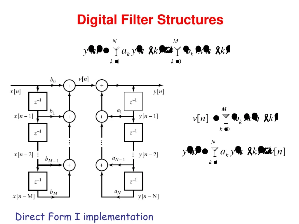
Digital Filter Structures. Direct Form I implementation. On the z-domain or equivalently. By changing the order of H 1 and H 2 , onsider the equivalence on the z-domain: where Let Then. In the time domain, We have the following equivalence for implementation:. We assume M=N here.

E N D
Digital Filter Structures Direct Form I implementation
On the z-domain or equivalently
By changing the order of H1 and H2, onsider the equivalence on the z-domain: where Let Then
In the time domain, We have the following equivalence for implementation: We assume M=N here
Note that the exactly the same signal, w[k], is stored in the two chains of delay elements in the block diagram. The implementation can be further simplified as follows: Direct Form II (or Canonic Direct Form) implementation
By using the direct form II implementation, the number of delay elements is reduced from (M+N) to max(M,N). Example: Direct form II implementation Direct form I implementation
Representing by signal-flow graph Example: the signal-flow graph of direct form II.
Cascade Form If we factor the numerator and denominator polynomials, we can express H(z) in the form: where M=M1+2M2 and N=N1+2N2, gk and gk* are a complex conjugate pair of zeros, and ck and ck* are a complex conjugate pair of poles. It is because that any N-th order real-coefficient polynomial equation has n roots, and these roots are either real or complex conjugate pairs.
A general form is where and we assume that MN. The real poles and zeros have been combined in pairs. If there are an odd number of zeros, one of the coefficients b2k will be zero. It suggests that a difference equation can be implemented via the following structure consisting of a cascade of second-order and first-order systems: cascade form of implementation (with a direct form II realization of each second-order subsystems)
Example: Cascade structure: direct form I implementation Cascade structure: direct form II implementation
Parallel Form If we represent H(z) by additions of low-order rational systems: where N=N1+2N2. If MN, then Np = MN. Alternatively, we may group the real poles in pairs, so that
Illustration of parallel-form structure for six-order system (M=N=6) with the real and complex poles grouped in pairs.
another alternation of the same system Hence, given a system function, there are many ways to implement it. There are equivalent when infinite-precision arithmetic is used. However, their behavior with finite-precision arithmetic can be quite different.
A non-computable system While the signal flow graph is an efficient way to represent a difference equation, not all of its instances are realizable: If a system function has poles, a corresponding signal flow graph will have feedback loops. A signal flow graph is computable if all loops contain at least one unit delay element. Eg. Computable systems
Circular Convolution (for DFT) • Time-domain convolution implies frequency domain multiplication. This property is valid for continuous Fourier transform, Fourier series, and DTFT, but is not exactly true for DFT. • The DFT pair considered hereafter (following Openheim’s book, where the 1/N is put on the inverse-transform side): where WN = ej2/N is a root of the equation WN=1.
Circular Convolution (for DFT) • For DFT, time domain circular convolution implies frequency domain multiplication, and vice versa. • Consider a periodic sequence. Its DTFT is both periodic and discrete in frequency. Multiplication in the frequency domain results in a convolution of the two corresponding periodic sequences in the time domain. Now let’s consider a single period of the resulted sequence. Since the two sequences are both periodic, the convolution appears as ‘folding’ the rear of a sequence to the front one by one, and superimposing the inner products so obtained, in a single period.
circular convolution Circular convolution (definition) • Symbol for representing circular convolution: or N . If the DFT of x1[n], x2[n], and x3[n] are X1[k], X2[k], and X3[k], respectively. • Time domain circular convolution implies frequency domain multiplication: • Time domain multiplication implies frequency domain circular convolution (with 1/N amplitude reduction):
Example: circular convolution with a delayed impulse sequence
Example: circular convolution of two rectangular pulses N-point circular convolution of two sequences of length N.
Example: circular convolution of two rectangular pulses (continue) Given two sequences of length L, assume that we add L zeros on its end, making an N=2L point sequence – referred to as zero padding N-point circular convolution of two sequences of length L, where N=2L.
N-point circular convolution of two sequences of length L, where N=2L (continue). Note that by zero padding, we can use circular convolution to compute convolution of two finite length sequences.
Some other properties involving circulation: • Time domain circular shift implies frequency domain phase shift: Duality property of DFT: • Since DFT and IDFT has very similar form, we have a duality property for DFT: If Then
Sampling the DTFT spectrum We have seen that, for an M-point sequence, if we uniformly sample M points in its DTFT spectrum within [0, 2], we can equivalently obtain its DFT. • What happen when we sample N points in the frequency domain [0, 2], instead of M points? Let the samples be We will have the following property: which means that “frequency-domain sampling implies time domain aliasing.” • when N M, no aliasing will happen, and particular when N=M, we obtain DFT. • when N < M, aliasing (of nonzero values) happens.
Linear Convolution Using DFT • Recall that linear convolution is when the lengths of x1[n] and x2[n] are L and P, respectively the length of x3[n] is L+P-1. • Thus a useful property is that the circular convolution of two finite-length sequences (with lengths being L and P respectively) is equivalent to linear convolution of the two N-point (N L+P1) sequences obtained by zero padding. • Another useful property is that we can perform circular convolution and see how many points remain the same as those of linear convolution. When P < L and an L-point circular convolution is performed, the first (P1) points are corrupted by circulation, and the remaining points from n=p1 to n=L1 (ie. The last LP+1 points) are not corrupted (ie., the last LP+1 points remain the same as the linear convolution result).
Block convolution (for implementing an FIR filter) • FIR filtering is equal to the linear convolution of a (possibly) infinite-length sequence. • To avoid delay in processing, and also to make efficient computation, we would like to segment the signal into sections of length L. Each L-length sequence can then be convolved with the finite-length impulse response and the filtered sections fitted together in an appropriate way. – called block convolution. • When each section is sufficiently large, we usually use circular convolution (instead of linear convolution) to compute each section. (since it will be shown that there are fast algorithms, fast Fourier transform (FFT), to compute circular convolutions highly efficiently) • Two methods for circular-convolution-based block convolution: Overlapping-add method and overlapping-save method.
Overlapping-add method (for implementing an FIR filter) When segmenting into L-length segments, the signal x[n] can be represented as where Because convolution is an LTI operation, it follows that where Since xr[n] is of length L and h[n] is of length P, each yr[n] has length (L+P1). So, we can use zero-padding to form two N point sequences, N=L+P1, for both xr[n] and h[n]. Performing N-point circular convolution (instead of linear convolution) to compute yr[n].
For example, consider two sequences h[n] and x[n] as follows.
Segmenting x[n] into L-length sequences. Each segment is padded by P1 zero values. Fir filtering by using the overlapping-add method.
Overlapping-save method (for implementing an FIR filter) Can we perform L-point circular convolution, instead of (L+P1)-point circular convolution? If a P-point sequence is circularly convolved with a P-point sequence (P<L), the first (P1) points of the result are incorrect, while the remaining points are identical to those that would be obtained by linear convolution. • Separating x[n] as overlapping sections of length L, so that each section overlaps the preceding section by (P1) points. Then
Example of overlapping-save method Decompose x[n] into overlapping sections of length L
Example of overlapping-save method (continue) Result of circularly convolving each section with h[n]. The portions of each filter section to be discarded in forming the linear convolution are indicated
See the following reference for the suggestion of L and P: M. Borgerding, “Turning Overlap-Save into a Multiband Mixing, Downsampling Filter Bank,” IEEE Signal Processing Magazine, pp. 158-161, 2006. Fast Fourier Transform (FFT) DFT pairs: WN = ej2/N is a root of the equation WN=1. It requires N2 complex multiplications and (N1)N complex additions for computation. Each complex multiplication needs four real multiplications and two real additions, and each complex addition requires two real additions. It requires 4N2 real multiplications and N(4N2) real additions.
Goertzel algorithm Since Define The above equation can be interpreted as a discrete convolution of the finite-duration sequence x[n], 0 n N1, with the sequence , which is the impulse response of the LTI system. Note that x[r] is nonzero only when 0 r < N. We can easily verify that
The Goertzel algorithm computes DFT by implementing the above LTI system. The system function is the z transform of The signal-flow graph of the LTI system for obtaining yk[n] is
vk[n] The implementation can be further simplified as Flow graph of second-order computation of X[k] (Goertzel algorithm)
Since we only need to bring the system to a state from which yk[n] can be computed, the complex multiplication by Wnk required to implement the zero of the system need not be performed at every iteration, but only after the N-th iteration, by the following difference equation: It requires 2 real multiplications and 4 real additions to compute vk[n] (that may be a complex sequence). The multiplication by Wnk is performed only when n=N, which requires 4 real multiplications and 4 real additions. Finally, a total of 2N+4 real multiplications and 4N+4 real additions are required. To compute all the X[k], k=0, …, N1, we need 2N(N+2) real multiplications and 4N(N+1) real additions, where the number of multiplications are reduced by almost a half. The Goertzel algorithm is usually used to compute X[k] for which only a single k or a small number of k values are needed.
Decimation-in-time FFT algorithm Most conveniently illustrated by considering the special case of N an integer power of 2, i.e, N=2v. Since N is an even integer, we can consider computing X[k] by separating x[n] into two (N/2)-point sequence consisting of the even numbered point in x[n] and the odd-numbered points in x[n]. or, with the substitution of variable n=2r for n even and n=2r+1 for n odd
Since That is, WN2 is the root of the equation WN/2=1 Consequently, Both G[k] and H[k] can be computed by (N/2)-point DFT, where G[k] is the (N/2)-point DFT of the even numbered points of the original sequence and the second being the (N/2)-point DFT of the odd-numbered point of the original sequence. Although the index ranges over N values, k = 0, 1, …, N-1, each of the sums must be computed only for k between 0 and (N/2)-1, since G[k] and H[k] are each periodic in k with period N/2.
Decomposing N-point DFT into two (N/2)-point DFT for the case of N=8
We can further decompose the (N/2)-point DFT into two (N/4)-point DFTs. For example, the upper half of the previous diagram can be decomposed as
Hence, the 8-point DFT can be obtained by the following diagram with four 2-point DFTs.
Finally, each 2-point DFT can be implemented by the following signal-flow graph, where no multiplications are needed. Flow graph of a 2-point DFT
Flow graph of complete decimation-in-time decomposition of an 8-point DFT.
In each stage of the decimation-in-time FFT algorithm, there are a basic structure called the butterfly computation: The butterfly computation can be simplified as follows: Flow graph of a basic butterfly computation in FFT. Simplified butterfly computation.
Flow graph of 8-point FFT using the simplified butterfly computation
In the above, we have introduced the decimation-in-time algorithm of FFT. Here, we assume that N is the power of 2. For N=2v, it requires v=log2N stages of computation. The number of complex multiplications and additions required was N+N+…N = Nv = N log2N. When N is not the power of 2, we can apply the same principle that were applied in the power-of-2 case when N is a composite integer. For example, if N=RQ, it is possible to express an N-point DFT as either the sum of R Q-point DFTs or as the sum of Q R-point DFTs. In practice, by zero-padding a sequence into an N-point sequence with N=2v, we can choose the nearest power-of-two FFT algorithm for implementing a DFT. The FFT algorithm of power-of-two is also called the Cooley-Tukey algorithm since it was first proposed by them. For short-length sequence, Goertzel algorithm might be more efficient.