Image Compression

1. Image Compression M.Sc. Nov.2015

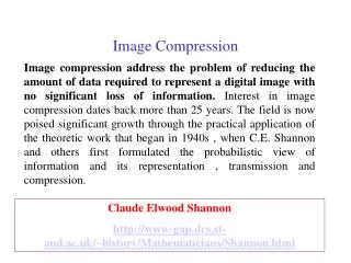
2. Image Compression Image compression involves reducing the size of image data file, while is retaining necessary information, the reduced file is called the compressed file and is used to reconstruct the image, resulting in the decompressed image. The original image, before any compression is performed, is called the uncompressed image file. The ratio of the original, uncompressed image file and the compressed file is referred to as the compression ratio. Compression Ratio = ------------------------------------ It is often written as SizeU: SizeC Uncompressed File Size …… Size U Compressed File Size ………………Size C

3. Examples Example:the original image is 256×256 pixel, single band (gray scale), 8-bit per pixel. This file is 65,536 bytes (64K). After compression the image file is 6,554 byte. The compression ratio is: SizeU: SizeC = this can be written as 10:1 This is called a “10 to 1” compression or a “10 times compression”, or it can be stated as “compressing the image to 1/10 original size. Another way to state the compression is to use the terminology of bits per pixel. For an N×N image Bit per Pixel =----------------------------------- =------------------------------- 8(Number of Bytes) Number of Bites Number of Pixels N * N

4. Examples Cont. Example: using preceding example, with a compression ratio of 65536/6554 bytes. We want to express this as bits per pixel. This is done by first finding the number of pixels in the image. 256×256 = 65,536 We then find the number of bits in the compressed image file 6554× (8 bit/byte) =52432 bits. Now, we can find the bits per pixel by taking the ratio 52432/65536=0.8 bit/ Pixel.

5. The reduction in file size is necessary to meet ) كمية البيانات)1- The bandwidth requirements for many transmission systems. 2-The storage requirements in computer data base. The amount of data required for digital images is enormous. For example, a single 512×512, 8-bit image requires 2,097,152 bits for storage. If we wanted to transmission this image over the World Wide Web, it would probably take minutes for transmission –too long for most people to wait. 512 ×512×8= 2,097,152. Example To transmit a digitized color scanned at 3,000×2,000 pixels, and 24 bits, at 28.8(kilobits/second), it would take about

6. Couple this result with transmitting multiple image or motion images, and the necessity of image compression can be appreciated. The key to a successful compression schema comes with the second part of the definition –retaining necessary information. To understand this we must differentiate between data and information. For digital images, data refer to pixel gray-level values the correspond to the brightness of a pixel at a point in space. Information is interpretation of the data in a meaningful way. Data are used to convey information, much like the way the alphabet is used to convey information via words. Information is an elusive concept, it can be application specific. For example, in a binary image that contains text only, the necessary information may only involve the text being readable, whereas for a medical image the necessary information may be every minute detail in the original image. .

7. There are two primary types of images compression methods and they are: Lossless Compression Lossy Compression. Lossless Compression This compression is called lossless because no data are lost, and the original image can be recreated exactly from the compressed data. For simple image such as text-only images. Lossy Compression. These compression methods are called Lossy because they allow a loss because they allow a loss in actual image data, so original uncompressed image can not be created exactly from the compressed file. For complex images these techniques can achieve compression ratios of 100 0r 200 and still retain in high – quality visual information. For simple image or lower-quality results compression ratios as high as 100 to 200 can be attained.

8. Input Image I(r,c) Output Image I(r,c) Encoding Preprocessing a. Compression Compressed File input Image I(r,c) Decoding Postprocessing b. Decompression Compression System Model The compression system model consists of two parts: Compressor and Decompressor. Compressor: consists of preprocessing stage and encoding stage. Decompressor: consists of decoding stage followed by a post processing stage, as following figure

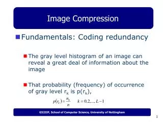
9. Lossles Compression Method Lossless compression methods are necessary in some imaging applications. For example with medical image, the law requires that any archived medical images are stored without any data loss. However lossless compression techniques may be used for both preprocessing and postprocessing in image compression algorithms. Additionally, for simple image the lossless techniques can provide perfect compression. An important concepts here is the ides of measuring the average information in an image, referred to as entropy. The entropy for N×N image can be calculated by this equation. .

10. (in bits per pixel) Where Pi = The probability of the ithgray level nk= the total number of pixels with gray value k. L= the total number of gray levels (e.g. 256 for 8-bits) Example: Let L=8, meaning that there are 3 bits/ pixel in the original image. Let that number of pixel at each gray level value is equal (they have the same probability) that is: Now, we can calculate the entropy as follows: This tell us that the theoretical minimum for lossless coding for this image is 8 bit/pixel • Note/ Log2(x) can be found by taking log10 and multiplying by 3.33

11. Why Data Compression? Graphical images in bitmap format take a lot of memory – e.g. For 3 Byte image the size (1024 x 768)pixels x 24 bits-per-pixel = 18,874,368 bits, or 2.4Mbytes. • But 120 Gbyte disks are now readily available!! • So why do we need to compress? • How long did that graphics-intensive web page take to download over your 56kbps modem?

12. • How many images could your digital camera hold? – Picture messaging? • CD (650Mb) can only hold less than 10 seconds of uncompressed video (and DVD only a few minutes) • We need to make graphical image data as small as possible for many applications

13. Types of Compression • Pixel packing • RLE (Run-length Encoding) • Dictionary-based methods • JPEG compression • Fractal Image Compression

14. Some factors to look out for: • Lossy or lossless compression? • What sort of data is a method good at compressing? • What is its compression ratio?

15. 1. Pixel Packing • Not a standard “data compression technique” but nevertheless a way of not wasting space in pixel data • e.g. – suppose pixels can take grey values from 0-15 – each pixel requires half a byte – but computers prefer to deal with bytes – two pixels per byte doesn’t waste space • Pixel packing is simply ensuring no bits are wasted in the pixel data • (Lossless if assumption true)

16. Pixel packing is not so much a method of data compression as it is an efficient way to store data in contiguous bytes of memory. In anther word is not a standard “data compression technique” it’s a way of not wasting space in pixel data • Most bitmap formats use pixel packing to conserve the amount of memory or disk space required to store a bitmap

17. If you are working with image data that contains four bits per pixel (suppose pixels can take grey values from 0-15). • you might find it convenient to store each pixel in a byte of memory, because a byte is typically the smallest addressable area of memory on most computer systems • by using this arrangement, half of each byte is not being used by the pixel data ( each pixel requires half a byte ) . • Ex: Image data containing 4096 4-bit pixels will require 4096 bytes of memory for storage, half of which is wasted.

18. To save memory, you could resort to pixel packing; instead of storing one 4-bit pixel per byte (two pixels per byte ). The size of memory required to hold the 4-bit, 4096-pixel image drops from 4096 bytes to 2048 bytes . • In the end doesn’t waste space

19. Pixel Packing Pixel-1 Pixel-2 4-bit unpacking pixel Pixel-3 Pixel-4 Pixel-6 Pixel-5 4-bit packing pixel

20. Cost of Compression • The tradeoff is faster read and write times versus reduced size of the image file. This is a good example of one of the costs of data compression. • Pixel packing may seem like common sense, but it is not without cost. • Memory-based display hardware usually organizes image data as an array of bytes, each storing one pixel or less. If this is the case, it will actually be faster to store only one 4-bit pixel per byte and read this data directly into memory in the proper format • rather than to store two 4-bit pixels per byte, which requires masking and shifting each byte of data to extract and write the proper pixel values.

21. Cost of Compression • In this case, the cost is in the time it takes to unpack each byte into two 4-bit pixels. • when decompressing image data: buffers need to be allocated and managed. • CPU-intensive operations must be executed and serviced

22. 2. Run-length encoding (RLE) is a very simple form of data compression in which runs of data (that is, sequences in which the same data value occurs in many consecutive data elements) are stored as a single data value and count, rather than as the original run. This is most useful on data that contains many such runs: for example, simple graphic images such as icons and line drawings.

23. For example, consider a screen containing plain black text on a solid white background. There will be many long runs of white pixels in the blank space, and many short runs of black pixels within the text. Let us take a hypothetical single scan line, with B representing a black pixel and W representing white: • WWWWWWWWWWWWBWWWWWWWWWWWWBBBWWWWWWWWWWWWWWWWWWWWWWWWBWWWWWWWWWWWWWW

24. If we apply the run-length encoding (RLE) data compression algorithm to the above hypothetical scan line, we get the following: 12WB12W3B24WB14W • Interpret this as twelve W's, one B, twelve W's, three B's, etc. Another example is this: AAAAAAAAAAAAAAA would encode as 15A AAAAAAbbbXXXXXt would encode as 6A3b5X1t So this compression method is good for compressing large expanses of the same color.

25. Run-length Encoding Simplest method of compression. How: replace consecutive repeating occurrences of a symbol by 1 occurrence of the symbol itself, then followed by the number of occurrences. The method can be more efficient if the data uses only 2 symbols (0s and 1s) in bit patterns and 1 symbol is more frequent than another

26. The Shannon-Fano Algorithm This is a basic information theoretic algorithm. A simple example will be used , to illustrate the algorithm: Symbol A B C D E Count 15 7 6 6 5 (sum=39) P (15/39)= 0.384 (7/39)=0.179 0.153 0.1530.1280

27. The Shannon-FanoAlgorithm cont. A 15 0.384 00 30 B 7 0.179 01 14 C 6 0.153 10 12 D 6 0.153 110 18 E 5 0.128 111 15 TOTAL (# of bits): 89

28. Huffman Coding A bottom-up approach 1. Initialization: Put all nodes in an OPEN list, keep it sorted at all times (e.g., ABCDE). 2. Repeat until the OPEN list has only one node left: (a) From OPEN pick two nodes having the lowest frequencies/probabilities, create a parent node of them. (b) Assign the sum of the children’s frequencies/probabilities to the parent node and insert it into OPEN. (c) Assign code 0, 1 to the two branches of the tree, and delete the children from OPEN.

29. Huffman cont.

30. Huffman Coding cont. • Symbol Count log(1/p) Code Subtotal (# of bits) A 15 1.38 0 15 B 7 2.48 100 21 C 6 2.70 101 18 D 6 2.70 110 18 E 5 2.96 111 15 TOTAL (# of bits): 87

31. Lempel-Ziv-Welch (LZW) Compression Algorithm • Introduction to the LZW Algorithm • Example 1: Encoding using LZW • Example 2: Decoding using LZW • LZW: Concluding Notes

32. Introduction to LZW • As mentioned earlier, static coding schemes require some knowledge about the data before encoding takes place. • Universal coding schemes, like LZW, do not require advance knowledge and can build such knowledge on-the-fly. • LZW is the foremost technique for general purpose data compression due to its simplicity and versatility. • It is the basis of many PC utilities that claim to “double the capacity of your hard drive” • LZW compression uses a code table, with 4096 as a common choice for the number of table entries.

33. Introduction to LZW (cont'd) • Codes 0-255 in the code table are always assigned to represent single bytes from the input file. • When encoding begins the code table contains only the first 256 entries, with the remainder of the table being blanks. • Compression is achieved by using codes 256 through 4095 to represent sequences of bytes. • As the encoding continues, LZW identifies repeated sequences in the data, and adds them to the code table. • Decoding is achieved by taking each code from the compressed file, and translating it through the code table to find what character or characters it represents.

34. LZW Encoding Algorithm 1 Initialize table with single character strings 2 P = first input character 3 WHILE not end of input stream 4 C = next input character 5 IF P + C is in the string table 6 P = P + C 7 ELSE 8   output the code for P 9 add P + C to the string table 10 P = C 11 END WHILE 12 output code for P

35. Example 1: Compression using LZW Example 1: Use the LZW algorithm to compress the string BABAABAAA

36. Example 1: LZW Compression Step 1 BABAABAAA P=A C=empty

37. Example 1: LZW Compression Step 2 BABAABAAA P=B C=empty

38. Example 1: LZW Compression Step 3 BABAABAAA P=A C=empty

39. Example 1: LZW Compression Step 4 BABAABAAA P=A C=empty

40. Example 1: LZW Compression Step 5 BABAABAAA P=A C=A

41. Example 1: LZW Compression Step 6 BABAABAAA P=AA C=empty

42. LZW Decompression • The LZW decompressor creates the same string table during decompression. • It starts with the first 256 table entries initialized to single characters. • The string table is updated for each character in the input stream, except the first one. • Decoding achieved by reading codes and translating them through the code table being built.

43. LZW Decompression Algorithm 1 Initialize table with single character strings 2 OLD = first input code 3 output translation of OLD 4 WHILE not end of input stream 5 NEW = next input code 6  IF NEW is not in the string table 7 S = translation of OLD 8   S = S + C 9 ELSE 10  S = translation of NEW 11 output S 12   C = first character of S 13   OLD + C to the string table 14 OLD = NEW 15 END WHILE

44. Example 2: LZW Decompression 1 Example 2: Use LZW to decompress the output sequence of Example 1: <66><65><256><257><65><260>.

45. Example 2: LZW Decompression Step 1 <66><65><256><257><65><260> Old = 65 S = A New = 66 C = A

46. Example 2: LZW Decompression Step 2 <66><65><256><257><65><260> Old = 256 S = BA New = 256 C = B

47. Example 2: LZW Decompression Step 3 <66><65><256><257><65><260> Old = 257 S = AB New = 257 C = A

48. Example 2: LZW Decompression Step 4 <66><65><256><257><65><260> Old = 65 S = A New = 65 C = A

49. Example 2: LZW Decompression Step 5 <66><65><256><257><65><260> Old = 260 S = AA New = 260 C = A

50. LZW: Some Notes • This algorithm compresses repetitive sequences of data well. • Since the codewords are 12 bits, any single encoded character will expand the data size rather than reduce it. • In this example, 72 bits are represented with 72 bits of data. After a reasonable string table is built, compression improves dramatically. • Advantages of LZW over Huffman: • LZW requires no prior information about the input data stream. • LZW can compress the input stream in one single pass. • Another advantage of LZW its simplicity, allowing fast execution.