Introduction to Integral Calculus

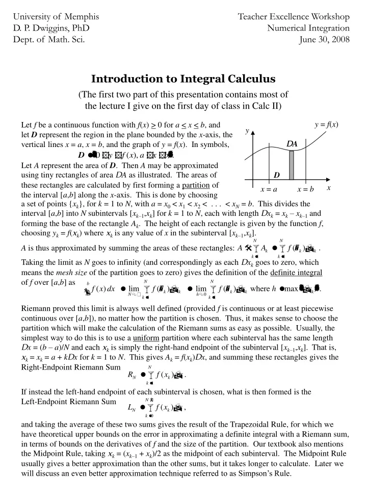
1. y = f(x) y DA D x x = a x = b University of MemphisD. P. Dwiggins, PhDDept. of Math. Sci. Teacher Excellence WorkshopNumerical IntegrationJune 30, 2008 Introduction to Integral Calculus (The first two part of this presentation contains most of the lecture I give on the first day of class in Calc II) Let f be a continuous function with f(x) > 0 for a<x<b, andlet D represent the region in the plane bounded by the x-axis, the vertical lines x = a, x = b, and the graph of y = f(x). In symbols, Let A represent the area of D. Then A may be approximated using tiny rectangles of area DA as illustrated. The areas of these rectangles are calculated by first forming a partition of the interval [a,b] along the x-axis. This is done by choosing a set of points {xk}, for k = 1 to N, with a = x0 < x1 < x2 < . . . < xN = b. This divides the interval [a,b] into N subintervals [xk–1,xk] for k = 1 to N, each with length Dxk = xk – xk–1 and forming the base of the rectangle Ak. The height of each rectangle is given by the function f, choosing yk = f(xk) where xk is any value of x in the subinterval [xk–1,xk]. A is thus approximated by summing the areas of these rectangles: Taking the limit as N goes to infinity (and correspondingly as each Dxk goes to zero, which means the mesh size of the partition goes to zero) gives the definition of the definite integral of f over [a,b] as Riemann proved this limit is always well defined (provided f is continuous or at least piecewise continuous over [a,b]), no matter how the partition is chosen. Thus, it makes sense to choose the partition which will make the calculation of the Riemann sums as easy as possible. Usually, the simplest way to do this is to use a uniform partition where each subinterval has the same length Dx = (b – a)/N and each xk is simply the right-hand endpoint of the subinterval [xk–1,xk]. That is, xk = xk = a + kDx for k = 1 to N. This gives Ak = f(xk)Dx, and summing these rectangles gives the Right-Endpoint Riemann Sum If instead the left-hand endpoint of each subinterval is chosen, what is then formed is the Left-Endpoint Riemann Sum and taking the average of these two sums gives the result of the Trapezoidal Rule, for which we have theoretical upper bounds on the error in approximating a definite integral with a Riemann sum, in terms of bounds on the derivatives of f and the size of the partition. Our textbook also mentions the Midpoint Rule, taking xk = (xk–1 + xk)/2 as the midpoint of each subinterval. The Midpoint Rule usually gives a better approximation than the other sums, but it takes longer to calculate. Later we will discuss an even better approximation technique referred to as Simpson’s Rule.

2. The Fundamental Theorem of Calculus Let f be a continuous function with f(x) > 0 for a<x<b, and define the area function A(t) for a<t<b in terms of the definite integral: Note A(a) = 0, and since f is nonnegative A(t) must be an increasing function (the area under the curve increases as t increases). We know from Calc I that if a differentiable function is increasing then its derivative must be positive. To determine whether or not A(t) is differentiable, we need to calculate the difference quotient: DA is calculated using the additivity of the definite integral: Note DA uses values of f(x) for x between t and t + Dt, so taking the limit as Dt goes to zero forces x to be equal to t. Thus, for Dt small enough, f(x) can be replaced by f(t), and so which means is approximatelyequal to f(t) when Dt is small enough, and since f is continuous this approximation gets better as Dt gets smaller. Thus, taking the limit as Dt goes to zero shows the area function is differentiable, with its derivative given byThis is the statement of the Fundamental Theorem of Calculus. In other words, if a function is constructed in terms of the definite integral for a continuous integrand f, then the constructed function is differentiable and its derivative is simply equal to f. Another way to state this is that the operations of integration and differentiation are inverse operations, i.e. they cancel each other out. This can be written symbolically as which is sometimes referred to as Version One of the Fundamental Theorem of Calculus. Another way to say the operations of calculating integrals and derivatives are inverse operations is to state that integration can be performed using antiderivatives, where “F is an antiderivative of f ” is true whenever f is the derivative of F. Lettinggives F as an antiderivative of f, since the Fundamental Theorem of Calculus states the derivative of F is equal to f. Using the additivity of the definite integral gives which is the statement of Version Two of the Fundamental Theorem of Calculus. If the Fundamental Theorem of Calculus is used to calculate definite integrals, then the techniques of integration basically involve methods for finding antiderivatives. This is not as easy as the problem of calculating derivatives, since the definition of the derivative (in terms of the limiting value of a difference quotient) always gives a way to calculate the derivative, but the definition of the definite integral (in terms of the limiting value of a Riemann Sum) does not give any way to calculate antiderivatives. Thus the only way to calculate antiderivatives is to study the rules for derivatives and then figure out how to write those rules backwards.

3. The Trapezoidal Rule If f(x) is continuous for a<x<b, the definite integral is well-defined, and if anantiderivative of f can be found then the integral can be evaluated using the FundamentalTheorem of Calculus. However, if f does not have an elementary antiderivative, then numerical techniques must be used to calculate the definite integral. The simplest way to approximate values of a function f is to use its linearization, and the simplest way to approximate the value of a definite integral is to use a piecewise-linear interpolation of f. Choose a uniform partition {xk} with a = x0 < x1 < . . . < xN = b, wherexk = xk–1 + Dx for k = 1, 2, …, N and Dx = (b – a)/N. Let yk = f(xk) for k = 0, 1, 2, …, N. The piecewise-linear function obtained by connecting the points {(xk , yk)} with straight line segments is called a linear spline for f. Each spline segment forms one side of a trapezoid with parallel sides along the vertical lines x = xk–1,x = xk, connected by the perpendicular “height” Dx. The vertical sides form the “bases” of the trapezoid, with lengths yk–1 and yk, and so the median of each trapezoid has length (yk–1+ yk)/2. Thus, the area of each trapezoid is calculated using median  height, or Note this is the same as saying each trapezoid has area AT = (AL + AR)/2, where AL = f(xk–1)Dx is the area of the rectangle using the left endpoint of each subinterval and AR = f(xk)Dx is the area of the rectangle using the right endpoint. Thus, the area calculated using the Trapezoidal Rule is the same as the average of the left-hand and right-hand Riemann Sums: T = (L + R)/2. Here is an example. Use the trapezoidal rule to approximate Using N = 4 gives Dx = (4 – 0)/4 = 1, forming the partition {x0, x1, x2, x3, x4} = {0, 1, 2, 3, 4}, with corresponding functional values {y0, y1, y2, y3, y4} = {0, 1, 4, 9, 16}. The left-hand Riemann sum is given by L = y0 + y1 + y2 + y3 = 14, and the right-hand sum is given byR = y1 + y2 + y3 + y4 = 30. Thus, T = (L + R)/2 = (14 + 30)/2 = 22, which approximates area A with error eT = | A – T | = 2/3 . There are two ways to improve this calculated result, i.e. so that the error of approximation becomes smaller. One way is to increase the number of points in the partition, and the other is to use a different technique of numerical integration. We will keep returning to this example so we can demonstrate and compare both approaches. Note that in calculating L + R every value of yk gets used twice except the first and last. Thus, another way to write an equation for the trapezoidal rule is to use

4. The Midpoint Rule The trapezoidal rule is obtained by averaging the values of y = f(x) at the endpoints of each subinterval [xk–1, xk] for a uniform partition {xk}. Another averaging method which may be used is to average the values of x in the partition rather than the values of y. That is, let The area elements used to make up M are all rectangles, and each such “midpoint rectangle” has area DA which is somewhere between the areas of the rectangles using the heights calculated at the endpoints of each subinterval, but DA is not halfway between these upper and lower rectangles, since averaging the heights gives the trapezoidal rule. However, if f is monotone, say strictly increasing on [a, b], then when the graph of f cuts into each rectangle at its midpoint the graph will be above the rectangle half the time and below the rectangle half the time, and so these positive and negative errors in area tend to cancel each other, often making the midpoint rule a better approximation than the trapezoidal rule. Continuing the example, use the midpoint rule to approximate Using N = 4 and the same partition {x0, x1, x2, x3, x4} = {0, 1, 2, 3, 4}, the midpoints of the subintervals are given by {0.5, 1.5, 2.5, 3.5), with corresponding functional values (y = x2){0.25, 2.25, 6.25, 12.25}. Since Dx = 1, simply summing these values gives M = 21, which approximates A with error eM = | A – M | = 1/3, half the error of the trapezoidal rule. Thus, the midpoint rule gives a better approximation than the trapezoidal rule, using the same partition rather than increasing the number of points. But that is not quite true, since calculating the midpoints of all the subintervals actually doubled the number of values of x being used, and the midpoint rule calculates y at each of these new values of x. That is, the amount of work required in using the midpoint rule with a partition of N points is about the same as the amount of work required to use the trapezoidal rule with 2N points. To illustrate this point, the table at right contains the work needed to calculate the value of T obtained from the trapezoidal rule with N = 8. Note this table contains both the original partition used for N = 4as well as the midpoints calculatedfor each of those subintervals. Thus, computing the midpoint rule along with the trapezoidal rule for a given value of N is the same amount of work as computing the value of T with 2N points, and this trapezoidal value has half the error of the midpoint rule value. These values have the sum14 + 21 = 35 (Note this is thesame as L + Mfor the partitionwith N = 4.) }

5. Error Bounds If the exact value for a definite integral is known, then we can measure the performance of a numerical technique of integration by comparing its calculated value with the actual value. But if we knew the exact value for an integral then we wouldn’t be performing numerical integration. If we don’t know the exact value, then we need a different way of measuring the error obtained from a numerical method. What needs to be done is to determine a theoretical estimate of the error bound, which does not give us the exact error (otherwise we would know the exact value of the integral), but gives an upper bound for the magnitude of the error. One way to compare two quantities without knowing their exact values is to compare their derivatives. Thus, one way to derive a theoretical error bound is to express the error between the exact value and the calculated value as a function of some quantity, and then see what conclusions can be drawn fromthe derivatives of this function. For example, we could first consider the area function which has the properties A(0) = 0 and A(x) = f(x). Next, we could consider the result H obtained fromsome numerical technique using a partition with mesh size h, and let H(x) denote the numerical result obtained by letting h = x/m for some positive integer m. We should then calculate a few derivatives of H and see how they compare with the derivativesof A. Once we observe what may be a useful relation between the derivatives of Hand A, we set E = A – H and see if properties of the derivatives of E will give us auseful upper bound for the size of E. To illustrate this approach, consider approximating A(x) using a single trapezoid. That is, let Dx = x and set Note that T(0) = 0, and so T (0) = f(0) = A(0) and But A(x) = f(x) implies A(x) = f (x), and so T (x) = ½ xf (x) + A(x). Now let H(x) = T(x) – A(x) so that H(x) = T (x) – A(x) = ½ xf (x). In this equation, let M be the value of f (x), so that H(x) = (M/2)x is true. But if H is linear in x, then H must be quadratic, so that H(x) = (M/4)x2 + C, with C = 0 because T (0) = A(0)  H (0) = 0. Integrating one more time finally gives H(x) = (M/12)x3, so that the error H = T – A in using a trapezoid with height h = x is proportional to the cube of h. Now, in computing the antiderivatives we held M constant, losing the information that M = f (x).However, if we had an upper bound for | f (x)| we would have an upper bound for M. Thus, wehave the theoretical error bound for estimating the area under a curve using a trapezoid as (continued on next page)

6. Error Bounds: Trapezoidal Rule vs Midpoint Rule Since there are N trapezoids in the trapezoidal rule using mesh size h = (b – a)/N, we have where M2 is an upper bound for | f (x)| over [a, b]. Thus, if the number of points in the partition used in the trapezoidal rule is doubled, then the error becomes four times smaller. If you use a computer program to calculate the trapezoidal rule using ten times as many points, then the error becomes one hundred times smaller. This sounds like a good result, and is pretty useful, but if you think about it that means if you have an answer accurate to four decimal places and you want the next two places then you need to use ten times as many points. Then if you want to go from six to eight decimal places you need ten times again as many points. Thus, while the trapezoidal rule is useful for estimating areas to two or three decimal places it isn’t very useful in getting much past that point. In order to step up to the next level of numerical integration we have to begin using non-linear approximation, and the simplest non-linear function is quadratic. This iscovered in the next section, but first let’s compare the two linear methods, trapezoidal rule versus midpoint rule. Let T be the trapezoidal rule with N points and uniform mesh size h, let M be the midpoint rule using the midpoints of the subintervals defined by the N given points, and let T2 denote the trapezoidal rule using the N given points along with the N calculated midpoints, so that T2 uses 2N points and has mesh size equal to h/2. Finally, let eT, eM, and e2 denote the respective errors. Then immediately we have the theoretical upper bound for e2 as which is one-fourth the theoretical upper bound for eT. This does not necessarily mean e2is equal to one-fourth of eT, but if f is flat enough so that f  doesn’t change very much then we can find some common value of M such that Now, T2 was calculated using all the values of f(x) used in calculating T, plus all the values of f(x) used in calculating M, so adding T + M involves summing all 2N of these values and multiplying the sum by h. This will actually give twice T2, since in calculating T2 the sum of the values of f(x) is multiplied by h/2. Thus, T + M = 2*T2, which gives M = 2*T2 – T and hence which means the midpoint rule gives about half the error of the trapezoidal rule. The presence of the minus sign means if T is an overestimate of A then M is an underestimate and vice versa, depending on whether f is concave up or down. If the graph of f fluctuates wildly enough that different values of M have to be used in estimating the different methods then these results won’t always hold, so that it is possible to have an example where T gives a better estimate than M. However, even when f is flat enough to guarantee M is better than T, the work involved in calculating M means you might as well go ahead and finish calculating T2, which usually has half again the error that M has.

7. Simpson’s Rule Let f be continuous on [a, b], and let {xk} be a uniform partition of [a, b] which uses an even number of points. Instead of joining each successive pair of points (xk–1, yk–1) and (xk, yk) with a straight line segment, Simpson’s rule takes the partition points three at a time and finds the parabolic arc which joins the three points. That is, given three consecutive values xk–, xk, xk+1 in the partition, find a quadratic function Q(x) such that Q(xk–1) = f(xk–1), Q(xk) = f(xk), and Q(xk+1) = f(xk+1). Then A is approximated by integrating Q. It makes no difference when looking at the general problem if everything is shifted along the x-axis, and the algebraic part of this discussion becomes much simpler if we choose as the three points in the partition x0 = –h, x1 = 0, and x2 = h, where h = (b – a)/N. Let Q(x) = Ax2 + Bx + C. Then Q(0) = C C = y1 = f(0). Similarly, Q(h) = Ah2 + Bh + C = y2 = f(h)  Ah2 + Bh = y2 – y1 and Q(–h) = Ah2 – Bh + C = y0 = f(–h)  Ah2 – Bh = y0 – y1 , and adding these two equations gives 2Ah2 = y2 + y0 – 2y1 . It turns out we don’t need B, since which gives S = (h/3)*(y0 + 4y1 + y2) as the area under the quadratic interpolation. To calculate the total approximation over [a, b], we use this rule to calculate S over [x0, x2], then over [x2, x4], and so forth, ending with [xN–2, xN], which is why N has to be even in order to use Simpson’s rule. In adding all these subvalues of S, we obtain the sum which finally gives Simpson’s rule, The theoretical error bound associated with Simpson’s rule is given by where M4 is an upper bound for the fourth derivative of f on [a, b]. The proof for this error bound is given in the project handout, but note that eS goes to zero at a rate proportional to 1/N4, which means doubling N makes the error sixteen times smaller, and using ten times as many points gives four more decimal places correct in the approximation. As noted last time, this method of quadratic approximation, along with its associated error bound, was known to mathematicians years before Simpson published his results. It is only because he included this rule in his calculus textbook, and also because his book became a standard reference in the British schools, that it became referred to as “Simpson’s rule.”But also as noted last time that’s okay because Simpson rarely gets credit for developingthe final version of what is now referred to as “Newton’s method.”

8. Our Example Revisited Return to the earlier example of using linear methods to approximate the value of the definite integral given at right. Note that f(x) = x2 f (x) = 2  M2 = 2  Thus, taking N = 4 gives (32/3)*(1/16) = 2/3, which is the exact value of the error found when using the trapezoidal rule with N = 4. Similarly taking N = 8 gives the trapezoidal error to be 1/6. Since we also found the midpoint error to be equal to 1/3, we have in this case that | A – M | = ½ | A – T | , | A – T2 | = ¼ | A – T | , and that the theoretical error estimates give the exact values of the errors. This is because the given function is quadratic, and so the second derivative is constant. In using the same partition to calculate Simpson’s rule, we have which gives the exact value of the integral. In fact Simpson’s rule would give the exact value just using N = 2, because Simpson’s rule uses quadratic approximation and in this case the integrand is already quadratic. Note this also matches the theoretical error bound because if f is quadratic then the fourth derivative is equal to zero. Note this is also true of any cubic polynomial, which therefore gives the surprising conclusion that Simpson’s method also gives the exact answer if f is any cubic polynomial. Here is another example. Use numerical methods to approximate the integral In this case we know the exact value of the integral, so what we are doing is using numerical integration to approximate the value of ln2 = 0.6931… . Using N = 8, calculate the results of the trapezoidal rule and Simpson’s rule, and compare both results with the approximate value 0.6931. Next, calculate the theoretical error bounds and check that both results are consistent with the theory. Finally, use the error bound equations to find out what value of N would be needed to approximate the value of ln2 to 8 decimal places using both methods.

9. Exercises # 1. (a) The function does not have an elementary antiderivative, and so numerical integration is the only way to evaluate the integral Using N = 4, calculate the values of T and S for this integral, i.e. use the trapezoidal rule and Simpson’s rule to approximate the integral. (b) In order to determine how good these approximations are, we need to find upper bounds on the derivatives of Calculate the derivatives off and show M2 = 2 and M4 = 12. (c) Use the results of part (b) to estimate the errors in the approximations from part (a), which thus gives a pretty good idea of the value of the integral. Finally, determine what value of N would be needed to calculate this integral accurately to six decimal places using Simpson’s rule. # 2. Consider the problem of evaluating the integral (a) Calculate the approximations obtained by using the trapezoidal rule withN = 4, the midpoint rule with N = 4, and the trapezoidal rule with N = 8. (b) Contrary to what is expected, you should find the three answers in part (a) are nowhere close to each other. Use a calculator or computer to view the graph of sin(100x2) for 1 <x< 2, and use the graph to explain why numerical integration is not going to work very well in this case. # 3. Although we usually assume a uniform partition when performing numerical integration, there are occasions where a non-uniform partition might be more useful. For example, consider the integral Show the partition {0.00, 0.21, 0.44, 0.69, 0.96, 1.00} gives Riemann sums where a calculator is not needed to find the values of f(xk), except for the final value which is just the square root of 2. Calculate the left and right Riemann sums and average them, which thus gives the result of the trapezoidal rule with a non-uniform partition. If you wanted to do a similar calculation which provided more accuracy, what new partition could you use? (Hint: consider the perfect squares which lie between 1000and 2000.)

10. University of MemphisD. P. Dwiggins, PhDDept. of Math. Sci. Teacher Excellence WorkshopNumerical IntegrationJune 30, 2008 Project Handout: Splines and Numerical Integration A spline is a function which is continuous on [a, b] and which is also analytic except on some partition {xk} of [a, b]. That is, the spline is analytic on each open subinterval xk–1 < x < xk , and the spline must be continuous at the endpoints, but it does not have to be differentiable at the endpoints. An interpolating spline for a continuous function f on [a, b] is a spline which agrees with f at each partition point for some partition {xk} of [a, b]. The term “spline” comes from the word used in naval ship construction, where the hull of the ship is bent into its proper shape by fitting it to a thin flexible piece of wood (the spline) which has the desired shape. Thus, a mathematical spline is a simple (piecewise polynomial) flexible function which can be “bent” to fit through any number of points on the graph of a given function. The goal in using interpolation as a technique of integration is to use a spline which is easy to integrate and whose integral serves as an approximation for the integral of f. In order for this technique to be useful there must also be some way to estimate the error between the approximation and the exact value. Usually this error bound will be expressed in terms of N (the number of points in the partition), and the splines which are useful have error bounds which go to zero at a rate proportional to some power of 1/N (higher powers are preferred since they cause the error to go to zero at a faster rate). A linear spline is one where the spline is linear on each subinterval, and so the graph consists of connecting the points {(xk , f(xk))} with straight line segments. (“Connect the Dots”) Using linear splines as a technique of numerical integration defines the Trapezoidal Rule. Similarly, Simpson’s Rule is constructed using quadratic splines, forming a sequence of parabolic arcs which interpolates f. It only takes two points to uniquely determine a line, but it requires three points to uniquely determine a parabola. Thus, in Simpson’s Rule the first parabola interpolates on {x0, x1, x2}, the second parabola interpolates on {x2, x3, x4} (which makes the spline continuous at x2), the third parabola interpolates on {x4, x5, x6} (which makes the spline continuous at x4), and so forth ending with the final parabola interpolating on {xN–2 , xN–1 , xN}, and so N must be even in order to use Simpson’s Rule. To extend this method, if N is a multiple of 3 then we could use cubic splines, interpolating on points four at a time (starting with {x0, x1, x2, x3}), and if N is a multiple of 4 we could use quartic splines, interpolating on points five at a time (starting with {x0, x1, x2, x3, x4}). The goal of this handout is to demonstrate how cubic and quartic splines are constructed,followed by a discussion of how theoretical error bounds may be determined. The readermay then pursue this further and get some ideas about quintic and hextic splines. Thereare general equations which show how to compute the coefficients for these higher-ordered splines, and these may be found in textbooks on numerical analysis under the heading of Polynomial Interpolation. You could also search for the topics Lagrange Interpolating Polynomial and the Newton-Cotes method of numerical integration for more informationon these topics.

11. Splines and Numerical Integration Page 2 In the presentation on the Trapezoidal Rule a proof of the error bound was given, but not a proof for the error bound in Simpson’s Rule. In constructing the quadratic splines, it is customary to shift the interval [a, b] so that it is centered at 0, becoming the interval [–h, h]. To help prepare for the steps used to prove the error bound for eS, let’s first redo the proof for eT in this centered-at-zero setting. First consider the area function which implies A(x) = f(x) – (–1)f(–x) = f(x) + f(–x), which gives A(0) = 2f(0).Thus, A(x) = f (x) – f (–x), which gives A(0) = 0, and in general so that A(n) = 0 when n is even, and A(n) = 2f(0) when n is odd. Now construct the trapezoidal area over the interval [–x, x], so that h = 2x and the area is given by T = h*(f(x)+f(–x))/2, or T(x) = x[f(x) + f(–x)]. Note in this setting T(x) is equal to x times the derivative of the area function. Thus, T(x) = xA(x)  T (x) = A(x) + xA(x)  T (x) – A(x) = xA(x) = x[f (x) – f (–x)]. Now invoke the Mean Value Theorem on f , finding c in [–x, x] such that Let M = f(c). Then f (x) – f (–x) = 2Mx  T (x) – A(x) = x*2Mx = 2Mx2, which upon integrating gives and since h = 2x  x = h/2, this gives Thus, the trapezoidal rule gives the area plus an error term on the order of h3, and the error is bounded because M<M2 = max | f (x) |. Now let’s try the same approach in trying to find an error bound for Simpson’s Rule. Dividing the interval [–x, x] into two parts (so that h = x), forming the partition {–x, 0, x}, Simpson’s Rule gives Taking derivatives gives (note S (0) = 2f(0) = A(0)), and (with S(0) = 0 because A(0) = 0), and finally Again invoke the Mean Value Theorem to find c in [–x, x] such that and since we have verified that S – A, S – A, and S – A are all equal to zero at x = 0, we can integrate three times to obtain (continued on next page)

12. Splines and Numerical Integration Page 3 Thus, over a subinterval with partition points {a, a + h, a + 2h}, the error between Simpson’s Rule and the actual area is given by where M is equal to the value of the fourth derivative of f at some point. Taking M4 as an upper bound for M, setting h = (b – a)/N, and multiplying by N/2 (the number of quadratic subintervals) gives as the theoretical error bound for Simpson’s Rule. Note that if p(x) is a cubic polynomial then p(4) = 0, and so eS = 0 if Simpson’s Rule is used to integrate a cubic polynomial. For example, integrating p(x) = 15x – x3 for 1 <x< 5 gives while Simpson’s Rule gives S = (2/3)[p(1) + 4p(3) + p(5)] = (2/3)(14 + 4(18) – 50) = (2/3)(36) = 24  What this means is that if we try to construct a technique of numerical integration using cubic splines, we should not expect any great improvement over quadratic splines since the quadratic splines can already be used to calculate the integrals obtained from the cubic splines. The only source of reducing the error in going to cubic splines is that oneach subinterval they interpolate on one additional partition point, which may give a slight reduction in error but not very much. If we try to extend the method for Simpson’s Rule to cubic splines, the first thing to do is divide the interval [–x, x] into three parts and then find the cubic polynomial which agrees with f at ± x and at ± x/3. This part is left as an exercise, as is the result that integrating the cubic spline gives U(x) = (x/4)[f(–x) + 3f(–x/3) + 3f(x/3) + f(x)] as the approximation forthe exact area A(x). Now, for Simpson’s Rule, taking three derivatives of S(x) got us down to having at which point we could invoke the Mean Value Theorem to obtain an upper bound involving f (4)(x). However, for the cubic spline it will take us four derivatives to get U (4)(x) – A(4)(x) in terms of A(5)(x) = f (4)(x) + f (4)(–x), and in this case the sign between the values of f(4) is + instead of –, and so we can’t invoke the Mean Value Theorem at this step. Thus, the best we can do is to express the cubic error bound in terms of the fourth derivative of f, and also on the order of h5, the same as for Simpson’s Rule. In fact, the error bound for U – A can be given as (3/80)M4h5 (I am leaving the proof as another exercise because it is similar to that for quartic splines, which is coming up next), and after setting h = (b – a)/N and multiplying by N/3 (the number of pieces of the cubic spline when the partition has N points) the total error for the cubic spline has as its upper bound (M4/80)(b – a)5/N4. Comparing this with the error bound for Simpson’s Rule, eS< (M4/180)(b – a)5/N4, it is seen the error involved using cubic splines for numerical integration can be almost 2.5 times more than the error involved in using Simpson’s Rule. Thus, while cubic splines have applications in other areas of mathematics, they are not very useful for numerical integration.

13. Splines and Numerical Integration Page 4 For completeness, here is a proof of the error bound when quartic splines are used for numerical integration. Form a partition of [a, b] using N points, where N is a multiple of 4. Take the problem of finding a quartic polynomial which interpolates on the first four points {a, a + h, a + 2h, a + 3h, a + 4h} in the partition, and shift it along the x-axis to perform the equivalent problem on [–x, x] with the partition {–x, –x/2, 0, x/2, x} (h = x/2). If P(x) = Ax4 + Bx3 + Cx2 + Dx + E then which means we don’t have to find B and D. Also, P(0) = E and P agrees with f at 0, and soE = f(0). Using P(± x) = f(± x) gives the two equations Ax4 + Bx3 + Cx2 + Dx = f(x) – f(0) andAx4 – Bx3 + Cx2 – Dx = f(–x) – f(0). Adding these equations gives 2Ax4 + 2Cx2 = f(x) + f(–x) – 2f(0).Similarly, using P(± x/2) = f(± x/2) gives the equation (1/8)Ax4 + (1/2)Cx2 = f(x/2) + f(–x/2) – 2f(0). Solving the two derived equations for Ax4 and Cx2 givesAx4 = (2/3)f(x) + (2/3)f(–x) – (8/3)f(x/2) – (8/3)f(–x/2) + 4f(0)and Cx2 = (–1/6)f(x) + (–1/6)f(–x) + (8/3)f(x/2) + (8/3)f(–x/2) – 5f(0), and so calculating the value of (2/5)Ax5 + (2/3)Cx3 + 2Ex = (2x/15)[3Ax4 + 5Cx2 + 15E], the quartic area works out to be equal to (x/45)[7f(–x) + 32f(–x/2) + 12f(0) + 32f(x/2) + 7f(x)]. In terms of h and the values of y in the partition this quartic area is expressed as (2h/45)[7y0 + 32y1 + 12y2 + 32y3 + 7y4]. Now let A(x) denote the definite integral of f over [–x, x], so that A(x) = f(x) + f(–x), which also implies A(x/2) = f(x/2) + f(–x/2). Thus, the quartic area function can be written as The reason for stopping here is that we have reached the point where the function inside the square brackets has a derivative which is proportional to what is outside the brackets. That is, we have45R(6)(x) = x[G(x)] + 6G(x), where G(x) = 7A(6)(x) + A(6)(x/2).When you have z = x*y + y, then dy/dx = y = (z – y)/x, and so finding an upper bound on y gives an upper bound on (z – y)/x, which means if M is an upper bound for y then Mx gives an upper bound for z – y.Thus, we take the last derivative equation calculated above and subtract off A(6)(x): Note that A(6)(x) = f (5)(x) – f (5)(–x) so use the Mean Value Theorem to find c1 such that so that setting M1 = f (6)(c1) gives A(6)(x) = 2M1x. Similarly, find M2 = f (6)(c2) such that A(6)(x/2) = 2M2(x/2) = M2x. (continued on next page)

14. Splines and Numerical Integration Page 5 Thus, we have Suppose temporarily that f (6) is constant, i.e. f (6)(x) = M for every x, which then gives which upon integrating six times gives If f (6) is not constant we have to do more work but we can still obtain the above result for some M which is bounded by the maximum value of | f (6)(x)|. Taking this result, replacing h with (b – a)/N, and multiplying by N/4 finally gives as the error bound for quartic spline integration, where M6 is an upper bound for | f (6)(x)|. Example.f(x) = 1/x f (6)(x) = 720/x7 | f (6)(x)| < 720 for |x| > 1. Thus, taking M6 = 720, a = 1, and b = 2 gives eR< (1440/945)*(1/N6), so even just taking N = 4 gives an error of less than 0.01 when using the quartic spline to approximate ln2 = Also, in going from N = 4 to N = 8, the error becomes smaller by a factor of 46 > 4,000. Integration by quartic splines converges very quickly. Exercises. # 1. (a) Show that if Q(t) = At3 + Bt2 + Ct + D then (b) Use Q(± x) = f(± x) and Q(± x/3) = f(± x/3) to find equations eliminatingA and C, solve the resulting equations for Bx2 and D, and show the result from part (a) can be written as U(x) = (x/4)[f(x) + f(–x) + 3f(x/3) + 3f(–x/3)]. (c) Starting withU(x) = (x/4)[A(x) + 3A(x/3)], compute the first four derivatives of U, and show the final result can be written in the form 4U(4) = xG + 4G. (d) Write U(4) – A(4) in terms of f, and complete the proof of the error bound for numerical integration using cubic splines. # 2. (a) Explain why integration using quintic splines would not be an improvement over quartic splines. (b) Make a guess as to which derivative of f and which power of N would be used in the error bound for integration using hextic (sixth-degree) splines.

15. Splines and Numerical Integration Page 6 Exercises continued. # 3. (a) Show (b) Using N = 12, finish filling in the table below and calculate the approximations of p given by performing numerical integration on the integral in part (a) using trapezoids (T), Simpson’s rule (S), cubic splines (A3), and quartic splines (R). (c) It is a lot of work calculating the derivatives of but here is what I came up with: Use these values to verify the answers in part (b) agree with the theoretical error bounds. (d) Part (c) shows that, even though quartic splines use a higher power of N, if the derivatives of f are large then the quartic error may be about the size of the quadratic error. However, once N is large enough, then the higher-ordered splines become more useful. Use the theoretical error bounds to determine what values of N are needed to calculate p to 15 decimal places using T, S, and R as in part (b).