Download
1 / 41
520 likes | 846 Views
Discrete Cosine Transform. 1D DCT: expression of a set of n samples, f (x) as a sum of n cosine basis functions. * The cosine basis function for a set of 8 samples. u =4, -34. u =0, 438. u =1, -55. u =5, -132. u =2, 45. u =6, 34. u =7, 19. u =3, 52. u =0. u =4. u =1. u =5.

E N D
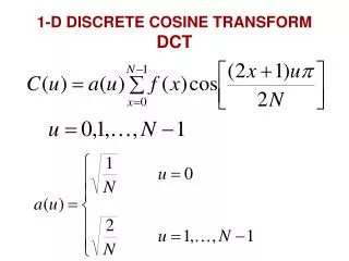
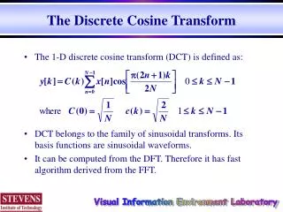
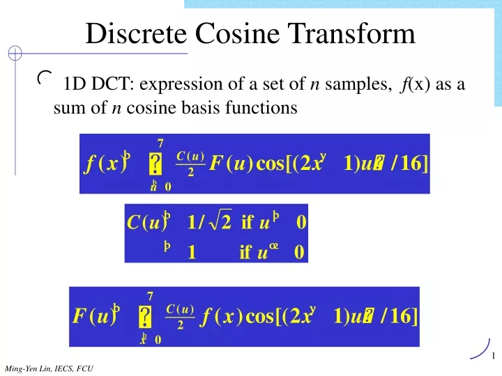
Discrete Cosine Transform • 1D DCT: expression of a set of n samples, f(x) as a sum of n cosine basis functions
* The cosine basis function for a set of 8 samples u=4, -34 u=0, 438 u=1, -55 u=5, -132 u=2, 45 u=6, 34 u=7, 19 u=3, 52
u=0 u=4 u=1 u=5 u=2 u=6 u=3 u=7
u=0 u=4 u=1 u=5 u=2 u=6 u=3 u=7
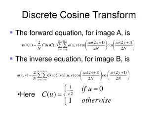
2D Discrete Cosine Transform • 2D DCT: transfer spatial domain to frequency domain • DC: F(0,0), average of f(x,y) • AC: other 63 coefficients
The 64 (8 x 8) DCT basis functions Entropy coding vs. transform coding
JPEG • Joint Photographic Expert Group • Continuous-tone image compression standard (color, grayscale) • Joint: collaboration between CCITT(ITU-T), ISO, IEC (ISO JTC1/SC2/WG10) • Official document: ISO/IEC 10918 -1, -2, -3 • History • 1987, selection process & narrow 12 proposal to 3 • 1988, select the DCT based method • 1988-90, defining, documenting, simulating, testing, validating • 1991, draft • 1992, International standard
Goals of JPEG • be at or near the state of the art of compression methods • be applicable to practically any kind of continuous-tone digital image • have tractable computational complexity to make feasible software & hardware implementation • 4 modes of operations • Lossy sequential encoding (baseline mode) • progressive encoding (multiple scan) • lossless encoding • hierarchical encoding (multiple resolution)
4 modes (illustration) Baseline sequential mode Expanded lossy DCT-based encoding (progressive)
3 4 7 初始圖 8 2 5 原圖 (original image) 預備編碼值 (coded result) 9 1 縮圖 (reduction) 6 擴展圖 (expansion) 4 modes (illustration) (cont’d) Hierarchical encoding
Major Steps of DCT-based modes • Encoder 8x8 blocks DCT-Based Encoder FDCT Quantizer Entropy Encoder Compressed Image Data Source Image Data Table Specification Table Specification
Major Steps of DCT-based modes (cont.) • Decoder DCT-Based Decoder Entropy Encoder Quantizer IDCT Compressed Image Data Reconstructed Image Data Table Specification Table Specification
Major Steps: Baseline Sequential Encoding U V YUV DC coeff AC coeff
色相轉換 R Cr G Cb B Y Color Model Transformation • Y = 0.299R +0.587G +0.114B • Cb = -0.168R -0.331G -0.499B • Cr = 0.500R -0.419G -0.081B
32 32 16 16 Subsampling (1/3) original
Preprocessing • Components, planes: 1 C 255 • in a C: different pixels (horizontal/vertical) allowed • Each pixel same depth 8, 12, 2 – 12 • component coding • Minimum coded unit (MCU): 4Y,1U,1V • Original sample value [0, 2 b-1] b bits used • 8-bits per sample in baseline mode • Shift to [-2 b-1, 2 b-1 ], center at 0 • b=8, [-128, 127] • Allow for low-precision calculation in DCT
Quantization • Quantization • to achieve further compression by representing DCT coefficients with no greater precision than is necessary • discard information which is not visually significant • Uniform quantization vs. Bit-rate control technique <e.g.> (110101)2= (53)10 quantization by 4 (1101)2 = (13)10 quantization by 8 (110)2 = (6)10
Quantization (cont.) • Adjust quantization step: tradeoff between compression ratio and image quality • Bit-rate control technique: • allocate more bits to the coefficients with large variances • division of DCT coefficients by corresponding quantizer step size • principle source of lossiness in DCT-based encoder
Quantization (Cont.) • Human eye is more sensitive to low frequencies than to high frequencies Luminance Quantization Table Chrominance Quantization Table ---------------------------------------------- ------------------------------------------------ 16 11 10 16 24 40 51 61 17 18 24 47 99 99 99 99 12 12 14 19 26 58 60 55 18 21 26 66 99 99 99 99 14 13 16 24 40 57 69 56 24 26 56 99 99 99 99 99 14 17 22 29 51 87 80 62 47 66 99 99 99 99 99 99 18 22 37 56 68 109 103 77 99 99 99 99 99 99 99 99 24 35 55 64 81 104 113 92 99 99 99 99 99 99 99 99 49 64 78 87 103 121 120 101 99 99 99 99 99 99 99 99 72 92 95 98 112 100 103 99 99 99 99 99 99 99 99 99 ----------------------------------------------- -----------------------------------------------
Zig-Zag Scan • transfer quantized coefficients from 2D to 1D sequence • transfer (8 x 8) to a (1 x 64) vector • Order coefficients in the order of increasing frequency • group low frequency coefficients in top of vector • Most high coeff are zero, result in most zero at the end of scan • Leading to higher entropy and run-length encode efficiency
Entropy Coding in JPEG • Additional lossless compression of DCT coefficients • Huffman Coding (baseline sequential) • Arithmetic Coding • pro: 5~10% better compression • con: complexity • Steps • conversion of quantized DCT coefficients to intermediate sequence of symbols • assignment of variable length codes to symbols
DPCM on DC Coefficients • DC component is large and varied, but often close to previous value. • DPCM (Differential Pulse Code Molulation) DC (DC) DCi-1 DCi 3 5 2 DCi=DCi-DCi-1
DPCM on DC Coefficients (cont.) • Step 1: DCi (Size, Amplitude) • Step 2: Encoding • size: • indicating size of VLI of amplitude, • VLC(huffman coding): input to encoder, application specific • amplitude • VLI (Variable Length Integer): hardwired into proposal
Size & Amplitude ------------------------------------ SIZE Value ------------------------------------ 1 -1, 1 (0,1) 2 -3, -2, 2, 3 (00, 01, 10, 11) 3 -7..-4, 4..7 (000, 001, 010, 011, 100,….) 4 -15..-8, 8..15 . . . . . . 10 -1023..-512, 512..1023 ------------------------------------ • Categorize DC values into SIZE (number of bits needed to represent) and actual bits.
RLC on AC Coefficients • 1 x 64 vector has lots of zeros in it • RLE: Run Length Encoding • Processing Steps • Step 1: AC (RunLength, Size), (Amplitude) • Step 2 • RunLength: VLC (Huffman coding) • Size: VLC • Amplitude: VLI
Lossless Mode • Predictive lossless coding (ratio 2-3 : 1)
Processing Steps of Lossless Mode Losseless Encoder Predictor Entropy Encoder Compressed Image Data Source Image Data Table Specification
Predictors for Lossless coding Selection Value Prediction 0 no prediction 1 A 2 B 3 C 4 A+B-C 5 A+(B-C)/2 6 B+(A-C)/2 7 (A+B)/2 Data unit in lossless Encoding is a single pixel C B A X Difference between X and predictor is entropy coded
Expanded lossy mode • Pixel depth of 12/ 8 bits • Huffman coding & Arithmetic coding • Progressive encoding & sequential encoding • Each component encoded in multiple scans instead of single scan • First scan rough, recognizable version for fast transmission, refined by succeeding scans • Need image sized buffer memory
Progressive Mode • DCT-based encoding • Difference: DCT Coefficients of each image component is encoded in multiple scan MSB Successive Approximation LSB Zig-Zag Sequence MSB Spectral Selection LSB Zig-Zag Sequence MSB (LSB): Most (Least) Significant Bit
Hierarchical Mode • Pyramid Coding at multiple resolution, each differ by factor 2 in either Hori/vertical T M O
Hierarchical encoding (1) • Filter and down sample original image by desired multiples of 2 in each dimension >>T • Encode the reduced size image T using one of sequential, progressive, lossless encoding • Decode the reduced image and interpolate and up-sample by a factor of 2 as a prediction of M • Get difference between Prediction and M, encode the difference using one the 3 coding schemes • Repeat steps 3 – 4 until full resolution encoded
Hierarchical encoding (2) • Encoded data of T is stored first, then encoded differences next • Useful when high resolution images be accessed by lower resolution device, no buffer to reconstruct full image then scale down • In browsing mode, low resolution data transmitted, displayed for fast response