Download
1 / 7
70 likes | 128 Views
Transient Conduction Approximation Calculator ( Lumped Capacitance and Analytical approximations). Spencer Ferguson and Natalie Siddoway April 7, 2014. Transient Conduction Approximations. Lumped Capacitance Assumes temperature uniformity throughout the body Valid for Bi < 0.1

E N D
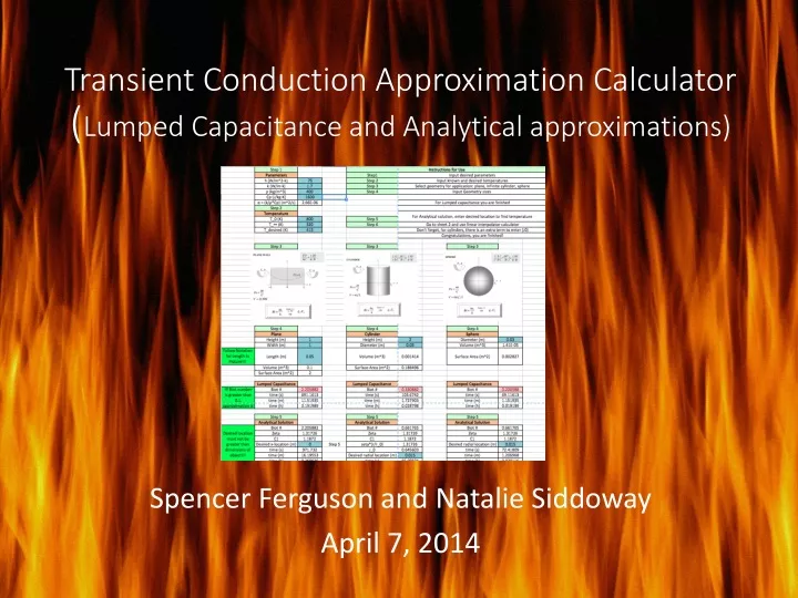
Transient Conduction Approximation Calculator(Lumped Capacitance and Analytical approximations) Spencer Ferguson and Natalie Siddoway April 7, 2014
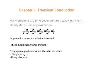
Transient Conduction Approximations • Lumped Capacitance • Assumes temperature uniformity throughout the body • Valid for Bi < 0.1 • Analytical approach • More accurate • More complex solution
Approximation Calculator • Calculates the time required for a body to reach a specified temperature • Lumped Capacitance: body temperature • Analytical method: any location on body • Inputs: h, k, ρ, c_p, temperatures, geometry, desired location (analytical only) • Output: approximated time to reach a temperature
Calculator layout Step 1: Input desired parameters Step 2: Input known and desired temperatures Step 3: Select geometry for application
Calculator layout Step 4: Input geometry sizes (follow layout) Step 5: Input desired location (analytical only) Step 6: For analytical, use linear interpolator to find c1 and ξ (also J_0 for cylinders) Evaluate solutions
Example Problem A sphere 30 mm in diameter initially at 800 K is quenched in a large bath having a constant temperature of 320 K with a convection heat transfer coefficient of 75 W/m^2-K. The thermophysical properties of the sphere material are: ρ=400 kg/m^3, c=1600 J/kg-K and k=1.7 W/m-K. Calculate the time required for the surface of the sphere to reach 415 K. Steps 1&2: Input desired parameters and temperatures Steps 3&4: Select geometry for application and input sizes
Example Problem A sphere 30 mm in diameter initially at 800 K is quenched in a large bath having a constant temperature of 320 K with a convection heat transfer coefficient of 75 W/m^2-K. The thermophysical properties of the sphere material are: ρ=400 kg/m^3, c=1600 J/kg-K and k=1.7 W/m-K. Calculate the time required for the surface of the sphere to reach 415 K. Steps 5&6: Input desired location, find c1 and ξ Evaluate solutions: • Lumped Capacitance Bi > 0.1, so lumped capacitance method is invalid • Analytical Fo > 0.2, so analytical approximation is valid


![Chapter 3: Unsteady State [ Transient ] Heat Conduction](https://cdn1.slideserve.com/2468294/chapter-3-unsteady-state-transient-heat-conduction-dt.jpg)