Download
1 / 47
880 likes | 2.71k Views
POLYMER CHEMISTRY . 2.1 Number average and weight average molecular weight 2.2 Polymer solutions 2.3 Measurement of number average molecular weight 2.4 Measurement of weight average molecular weight 2.5 Viscometry 2.6 Molecular weight distribution.

E N D
POLYMER CHEMISTRY 2.1 Number average and weight average molecular weight 2.2 Polymer solutions 2.3 Measurement of number average molecular weight 2.4 Measurement of weight average molecular weight 2.5 Viscometry 2.6 Molecular weight distribution Chapter 2. Molecular Weight and Polymer Solutions
2.1 Number Average and Weight Average Molecular Weight A. The molecular weight of polymers a. Some natural polymer (monodisperse) : All polymer molecules have same molecular weights. b. Synthetic polymers (polydisperse) : The molecular weights of polymers are distributed c. Mechanical properties are influenced by molecular weight much lower molecular weight ; poor mechanical property much higher molecular weight ; too tough to process optimum molecular weight ; 105 -106 for vinyl polymer 15,000 - 20,000 for polar functional group containing polymer (polyamide) POLYMER CHEMISTRY
B. Determination of molecular weight • Absolute method : • mass spectrometry • colligative property • end group analysis • light scattering • ultracentrifugation. • b. Relative method : solution viscosity • c. Fractionation method : GPC POLYMER CHEMISTRY
C. Definition of average molecular weight a. number average molecular weight ( Mn) Mn= (colligative property and end group analysis) b. weight average molecular weight ( Mw) Mw= (light scattering) i i Ni N M WiMi Wi POLYMER CHEMISTRY Where Ni is the number of molecules or the number of moles of those molecules- having molecular weight Mi. NiMi=Wi dn/dc : 농도변화에 따른 굴절률의 변화값
c. z average molecular weight ( MZ ) MZ= (ultracentrifugation) d. general equation of average molecular weight : M = ( a=0 , Mn a=1 , Mw a=2 , Mz ) e. Mz > Mw > Mn C. Definition of average molecular weight NiMi2 NiMi3 NiMia+1 NiMia POLYMER CHEMISTRY
Viscosity average molecular weight ( M) GPC-평균분자량, ( MGPC) Ostwald viscometers measure the viscosity of a fluid with a known density A typical Waters GPC instrument including A. sample holder, B.Column C.Pump D. Refractive Index Detector E. UV-vis Detector Schematic of pore vs. analyte size
D. Polydispersity index : width of distribution polydispersity index (PI) = Mw / Mn ≥ 1 POLYMER CHEMISTRY
E. Example of molecular weight calculation a. 9 moles, molecular weight (Mw) = 30,000 5 moles, molecular weight (Mw) = 50,000 (9 mol x 30,000 g/mol) + (5 mol x 50,000 g/mol) Mn= = 37,000 g/mol 9 mol + 5 mol 9 mol(30,000 g/mol)2 + 5 mol(50,000 g/mol)2 Mw = = 40,000 g/mol 9 mol(30,000 g/mol) + 5 mol(50,000 g/mol) POLYMER CHEMISTRY
= 35,000 g/mol 9 g + 5 g = 37,000 g/mol Mn= (9 g/30,000 g/mol) + (5 g/50,000 g/mol) (9 g/30,000 g/mol) + (5 g/50,000 g/mol) Mw = 9 g + 5 g POLYMER CHEMISTRY E. Example of molecular weight calculation b. 9 grams, molecular weight ( Mw) = 30,000 5 grams, molecular weight ( Mw ) = 50,000
a. number average molecular weight ( Mn) b. weight average molecular weight ( Mw) 강릉, 동해, 속초, 양양의 인구를 각각 700,000 + 10,000+ 12,000+ 1,500=723,500 723,500/4=180, 875 (수평균 인구수) 강릉 700,000 X 700,000/723,500= 700,000 X0.9675 = 677,263.3 동해 10,000 X 10,000/723,500= 10,000X0.0138 =138.2 속초 12,000 X 12,000/723,500= 12,000X0.0166=199.0 양양 1,500 X 1,500/723,500= 1,500X0.00207=3.2 677,263.3+ 138.2+199.0+3.2=677,603.7 677,600
2.2 Polymer Solutions A. Process of polymer dissolution : two step first step : the solvent diffuses into polymer masses to make a swollen polymer gel second step : swollen polymer gel breaks up to solution POLYMER CHEMISTRY
2.2 Polymer Solutions B. Thermodynamics of solubility : Gibb's free energy relationship G =H - TS ΔG < 0 : spontaneously dissolve T and ΔS are always positive for dissolving process. Conditions to be negative ΔG, ΔH must be negative or smaller than TΔS. POLYMER CHEMISTRY
C. Solubility parameter : δ Hmix=Vmix[( )1/2-()1/2]212 12= volume fraction ΔE1/V1, ΔE2/V2 = cohesive energy densities (분자를 이웃분자와 떨어뜨리는데 필요한 에너지) δ1,δ2 = solubility parameter δ1, δ2 = ( )1/2 Hmix= Vmix(δ1 – δ2)212 E = Hvap- RT 휘발성화홥물 ΔE1/V1 Vs Hvap- δ1 = ( )1/2 if δ1= δ2, then Hmix= 0 E1 E2 V1 V2 E V H vap - RT V POLYMER CHEMISTRY
D. Small's and Hoy's G parameter a. Small(designated G derived from Heat of vaporization, Table 2.1) δ = ( d : density , M : molecular weight of unit ) ex) polystyrene δ = = 9.0 b. Hoy(designated G based on vapor pressure measurement, Table 2.1) δ = ex) polystyrene : δ = dG M 1.05(133+28+735) 104 dG M 1.05[131.5+85.99+6(117.1)] = 9.3 104 POLYMER CHEMISTRY
E. Hydrodynamic volume of polymer molecules in solution. to be depended on followings r 2 = ro22 s2=so22 (r2)1/2 = (ro2)1/2 • polymer-polymer interaction • b. solvent-solvent interaction • c. polymer-solvent interaction • d. polymer structure ( branched or not ) • e. brownian motion • r = end-to-end distance • s = radius of gyration Figure 2.1 Coil molecular shape ro so: unperturbed dimension, 용매의영향을배제한고분자의크기 α(expansion factor) The greater the value of α, the ‘better’ the solvent α = 1, 'ideal' statistical coil.
2.2 Polymer Solutions F. theta (θ) temperature and theta (θ) solvent The lowest temperature at which α=1 : theta (θ) temperature blink The solvent satisfied this condition : theta (θ) solvent point G. Flory-Fox equation : The relationship among hydrodynamic volumes, intrinsic viscosity and molecular weight [η] : intrinsic viscosity M : average molecular weight : proportionality orFlory constant (3×1024/mol) r : end-to-end distance (r2)3/2 [η] = M POLYMER CHEMISTRY
2.2 Polymer Solutions H. Mark-Houwink-Sakurada equation : The relationship between intrinsicviscosity and molecular weight [η] : intrinsic viscosity K , a : constant for specific polymer and solvent M : average molecular weight I. Important properties of polymer solution : solution viscosity a. paint spraying and brushing b. fiber spinning [η] = KMa POLYMER CHEMISTRY
2.3 Measurement of Number Average Molecular Weight 2.3.1 End-group Analysis A. Molecular weight limitation up to 50,000 B. End-group must have detectable species a. vinyl polymer : -CH=CH2 b. ester polymer : -COOH, -OH c. amide and urethane polymer : -NH2, -NCO d. radioactive isotopes or UV, IR, NMR detectable functional group POLYMER CHEMISTRY
2.3 Measurement of Number Average Molecular Weight 2 x 1000 x sample wt C. Mn = meq COOH + meq OH D. Requirement for end group analysis 1. The method cannot be applied to branched polymers. 2. In a linear polymer there are twice as many end of the chain and groups as polymer molecules. 3. If having different end group, the number of detected end group is average molecular weight. 4. End group analysis could be applied for polymerization mechanism identified E. High solution viscosity and low solubility : Mn = 5,000 ~ 10,000
FIGURE 2.2 Schematic representation of a membrane osmometer.
2.3.2 Membrane Osmometry A. According to van't Hoff equation limitation of : 50,000 ~ 2,000,000 The major error arises from low-molecular-weight species diffusing through the membrane. RT )C=0 = + A2C ( c Mn FIGURE 2.3 Automatic membrane osmometer [Courtesy of Wescan Instruments, Inc.]
FIGURE 2.4. Plot of reduced osmotic pressure (/c) versus concentration (c). /c RT Mn Slope = A2 C POLYMER CHEMISTRY
2.3.3 Cryoscopy and Ebulliometry A. Freezing-point depression (Cryoscopy) Tf : freezing-point depression, C : the concentration in grams per cubic centimeter R : gas constant T : freezing point Hf: the latent heats of fusion A2 : second virial coefficient RT2 Tf + A2C ( )C=0 = Hf Mn C POLYMER CHEMISTRY
2.3.3 Cryoscopy and Ebulliometry B. Boiling-point elevation (Ebulliometry) Tb : boiling point elevation Hv : the latent heats of vaporization We use thermistor to major temperature. (1×10⁻⁴℃) limitation of Mn : below 20,000 RT2 Tb + A2C ( )C=0 = C HvMn POLYMER CHEMISTRY
2.3.4 Vapor Pressure Osmometry The measuring vapor pressure difference of solvent and solution drops. λ : the heat of vaporization per gram of solvent m : molality limitation of Mn : below 25,000 Calibration curve is needed to obtain molecular weight of polymer sample Standard material : Benzil RT2 T = ( )m 100 POLYMER CHEMISTRY The Wescore model 5500 Vapor Pressure Osmometer
2.3.5 Mass spectrometry A. Conventional mass spectrometer for low molecular-weight compound energy of electron beam : 8 -13 electron volts (eV) POLYMER CHEMISTRY
B. Modified mass spectrometer for synthetic polymer a. matrix-assisted laser desorption ionization mass spectrometry (MALDI-MS) b. matrix-assisted laser desorption ionization time-of-flight (MALDI-TOF) c. soft ionization sampling : polymers are imbedded by UV laser absorbable organic compound containing Na and K. d. are calculated by using mass spectra. e. The price of this mass is much more than conventional mass. f. Up to = 400,000 for monodisperse polymers. POLYMER CHEMISTRY
FIGURE 2.5. MALDI mass spectrum of low-molecular-weight poly(methyl methacrylate). POLYMER CHEMISTRY
2.3.6 Refractive Index Measurement A. The linear relationship between refractive index and 1/Mn . B. The measurement of solution refractive index by refractometer. C. This method is for low molecular weight polymers. D. The advantage of the method is simplicity. POLYMER CHEMISTRY
2.4 Measurement of Weight Average Molecular Weight 2.4.1 Light Scattering A. The intensity of scattered light or turbidity(τ) is depend on following factors a. size b. concentration c. polarizability d. refractive index e. angle f. solvent and solute interaction g. wavelength of the incident light POLYMER CHEMISTRY http://www.mals.co.kr/
g. wavelength of the incident light C : concentration no: refractive index of the solvent λ : wavelength of the incident light No : Avogadro's number dn/dc : specific refractive increment P() : function of the angle,θ A2 : second virial coefficient Zimm plot (after Bruno Zimm) : double extrapolation of concentration and angle to zero (Fig 2.6) 1 Hc + 2A2C = MP() = HcMW 32 No2(dn/dc)2 H = 3 4No POLYMER CHEMISTRY
FIGURE 2.6. Zimm plot of light-scattering data. Hc C=0 Experimental 1 Extrapolated Mw sin2/2 + kc POLYMER CHEMISTRY
2.4.1 Light Scattering B. Light source High pressure mercury lamp and laser light. C. Limitation of molecular weight( ) : 104~107 FIGURE 2.7. Schematic of a laser light-scattering photometer. POLYMER CHEMISTRY
2.4.2 Ultracentrifugation A. This technique is used a. for protein rather than synthetic polymers. b. for determination of Mz B. Principles : under the centrifugal field, size of molecules are distributed perpendicularly axis of rotation. Distribution process is called sedimentation. POLYMER CHEMISTRY Air-driven, vacuum-type ultracentrifuge
2.5 Viscometry A. IUPAC suggested the terminology of solution viscosities as following. Relative viscosity :단위없음 >1 : solution viscosity o: solvent viscosity t : flow time of solution t o: flow time of solvent Specific viscosity :단위없음 Reduced viscosity : Inherent viscosity : Intrinsic viscosity : t - to - o sp = rel - 1 = = t o to rel = = o to C:고분자용질의 농도 g/cm3 , g/dL sp rel - 1 rel = = c sp c [] = ( )c=o=(ηinh)C = 0 c In rel inh = c POLYMER CHEMISTRY g/cm3
FIGURE 2.8. Capillary viscometers : (A) Ubbelohde, and (B) Cannon-Fenske. POLYMER CHEMISTRY 일정한 농도,온도(0.5 g/100mL, 30.0±0.001 oC)
B. Mark-Houwink-Sakurada equation [η] = KMa log[η] = logK + alogMv (K, a : viscosity-Molecular weight constant, table2.3) Mv is closer to Mw than Mn Mw> Mv > Mn POLYMER CHEMISTRY
TABLE 2.3. Representative Viscosity-Molecular Weight Constantsa Solvent Cyclohexane Cyclihexane Benzene Decalin Benzyl alcohol Cyclohexanone Toluene Toluene DMFg DMF 1-Chlorobutane 1-Chlorobutane M-Cresol M-Cresol Temperature, oC 35 d 50 25 135 155.4d 20 30 30 25 25 30 30 25 25 Molecular Weight Range 10-4 8-42e 4-137e 3-61f 3-100e 4-35e 7-13f 5-50f 5-16f 5-27e 3-100f 5-55e 4.18-81e 0.04-1.2f 1.4-5f Polymer Polystyrene (atactic)c Polyethylene (low pressure) Poly(vinyl chloride) Polybutadiene 98% cis-1,4, 2% 1,2 97% trans-1,4, 3% 1,2 Polyacrylonitrile Poly(methyl methacrylate-co-styrene) 30-70 mol% 71-29 mol% Poly(ethylene terephthalate) Nylon 66 ab 0.50 0.599 0.74 0.67 0.50 1.0 0.725 0.753 0.81 0.75 0.67 0.63 0.95 0.61 Kb 103 80 26.9 9.52 67.7 156 13.7 30.5 29.4 16.6 39.2 17.6 24.9 0.77 240 aValue taken from Ref. 4e. bSee text for explanation of these constants. cAtactic defined in Chapter 3. d temperature. eWeight average. fNumber average. gN,N-dimethylformamide. POLYMER CHEMISTRY
2.6 Molecular Weight Distribution 2.6.1 Gel Permeation Chromatography (GPC) A. GPC or SEC (size exclusion chromatography) a. GPC method is modified column chromatography. b. Packing material: Poly(styrene-co-divinylbezene), glass or silica bead swollen and porous surface. c. Detector : RI, UV, IR detector, light scattering detector d. Pumping and fraction collector system for elution. e. By using standard (monodisperse polystyrene), we can obtain Mn , Mw . POLYMER CHEMISTRY
FIGURE 2.9. Schematic representation of a gel permeation chromatograph. POLYMER CHEMISTRY
FIGURE 2.10. Typical gel permeation chromatogram. Dotted lines represent volume “counts.” Detector response Baseline Elution volume (Vr) (counts) POLYMER CHEMISTRY
FIGURE 2.11. Universal calibration for gel permeation chromatography. THF, tetrahydrofuran. Log([η]M) 109 108 Polystyrene (linear) Polystyrene (comb) Polystyrene (star) Heterograft copolyner Poly (methyl methacrylate) Poly (vinyl chloride) Styrene-methyl methacrylate graft copolymer Poly (phenyl siloxane) (ladder) Polybutadiene 107 106 105 18 20 22 24 26 28 30 Elution volume (5 ml counts, THF solvent) POLYMER CHEMISTRY
FIGURE 2.12. Typical semilogarithmic calibration plot of molecular weight versus retention volume. 106 Molecular weight (M) 105 104 103 Retention volume (Vr) (counts) POLYMER CHEMISTRY
B. Universal calibration method to be combined Mark-Houwink-Sakurada equation [η]1M1 = [η]2M2 1 K1 K2 logM2 = ( )log( ) + ( 1 + a1 )logM1 1 + a2 1 + a2 POLYMER CHEMISTRY
2.6.2 Fractional Solution Soxhlet-type extraction by using mixed solvent. Reverse GPC : from low molecular weight fraction to high molecular weight fraction Inert beads are coated by polymer sample. POLYMER CHEMISTRY
2.6.3 Fractional Precipitation Dilute polymer solution is precipitated by variable non-solvent mixture. Precipitate is decanted or filtered Reverse fractional solution : from high molecular weight fraction to low molecular fraction POLYMER CHEMISTRY
2.6.4. Thin-layer Chromatography (TLC) Alumina- or silica gel coated plate. Low cost and simplicity. Preliminary screening of polymer samples or monitoring polymerization processes. POLYMER CHEMISTRY