Download
1 / 40
400 likes | 563 Views
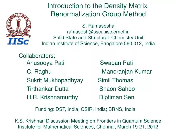
Introduction to the Density Matrix Renormalization Group Method S. Ramasesha ramasesh@sscu.iisc.ernet.in Solid State and Structural Chemistry Unit Indian Institute of Science, Bangalore 560 012, India. Collaborators: Anusooya Pati Swapan Pati

E N D
Introduction to the Density Matrix Renormalization Group Method S. Ramasesha ramasesh@sscu.iisc.ernet.in Solid State and Structural Chemistry Unit Indian Institute of Science, Bangalore 560 012, India Collaborators: Anusooya Pati Swapan Pati C. Raghu Manoranjan Kumar Sukrit Mukhopadhyay Simil Thomas Tirthankar Dutta Shaon Sahoo H.R. Krishnamurthy Diptiman Sen Funding: DST, India; CSIR, India; BRNS, India K.S. Krishnan Discussion Meeting on Frontiers in Quantum Science Institute for Mathematical Sciences, Chennai, March 19-21, 2012
o = tij (aiaj+ H.c.) + i ni † i <ij> HFull = Ho + ½ Σ [ij|kl] (EijEkl – jkEil) ijkl Eij = a†i,aj, Interacting One-Band Models • One-band tight binding model • Explicit electron – electron interactions essential for realistic modeling [ij|kl] = i*(1) j(1) (e2/r12) k*(2) l(2) d3r1d3r2 This model requires further simplification to enable routine solvability.
Zero Differential Overlap (ZDO) Approximation [ij|kl] = i*(1) j(1) (e2/r12) k*(2) l(2) d3r1d3r2 [ij|kl] = [ij|kl]ij kl
HHub = Ho + Σ Ui ni (ni - 1)/2 i Hubbard Model (1964) • Hückel model + on-site repulsions [ii|jj] = 0 for i j ; [ii|jj] = Ui for i=j • In the large U/t limit, Hubbard model gives the Heisenberg Spin-1/2 model
[ii|jj]parametrized byV( rij ) HPPP = HHub + Σ V(rij) (ni - zi) (nj - zj) i>j Pariser-Parr-Pople (PPP) Model ziare local chemical potentials. • Ohno parametrization: V(rij) = { [ 2 / ( Ui + Uj ) ]2 + rij2 }-1/2 • Mataga-Nishimoto parametrization: V(rij) = { [ 2 / ( Ui + Uj ) ] + rij }-1
12 V13 HPPP = Σ tij (aiσajσ+ H.c.) + Σ(Ui /2)ni(ni-1) + Σ V(rij) (ni - 1) (nj - 1) † <ij>σ i i>j Model Hamiltonian PPP Hamiltonian (1953)
Exact Diagonalization (ED) Methods • Fock space of Fermion model scales as 4n and of spin space as 2n n is the number of sites. • These models conserve total S and MS. • Hilbert space factorized into definite total S and MS spaces using Rumer-Pauling VB basis. • Rumer-Pauling VB basis is nonorthogonal, but complete, and linearly independent. • Nonorthogonality of basis leads to nonsymmetric Hamiltonian matrix • Recent development allows exploiting full spatial symmetry of any point group.
Necessity and Drawbacks of ED Methods • ED methods are size consistent. Good for energy gap extrapolations to thermodynamic or polymer limit. • Hilbert space dimension explodes with increase in no. of orbitals Nelectrons = 14, Nsites = 14, # of singlets = 2,760,615 Nelectrons = 16, Nsites = 16, # of singlets = 34,763,300 hence for polymers with large monomers (eg. PPV), ED methods limited to small oligomers. • ED methods rely on extrapolations. In systems with large correlation lengths, ED methods may not be reliable. • ED methods provide excellent check on approximate methods.
Implementation of DMRG Method • Diagonalize a small system of say 4 sites with two on the left and two on the right ● ● ● ● {|L>} = {| >, | >, | >, | >} 1 2 2’ 1’ H = S1 S2 + S2 S2’ + S2’ S1’|G> = CLR|L>|R> L R The summations run over the Fock space dimension L • Renormalization procedure for left block Construct density matrix L,L’ = RCLR CL’R Diagonalize density matrix > = Construct renormalization matrix OL = [· · · m] is L x m; m < L • Repeat this for the right block
HL = OL HLOL† ; HL is the unrenormalized L x L left-block Hamiltonian matrix, and HL is renormalized m x m left-block Hamiltonian matrix. • Similarly, necessary matrices of site operator of left block are renormalized. • The process is repeated for right-block operators with OR • The system is augmented by adding two new sites ● ● ● ● ● ● 1 2 3 3’ 2’ 1’ • The Hamiltonian of the augmented system is given by
Hamiltonian matrix elements in fixed DMEV Fock space basis • Obtain desired eigenstate of augmented system • New left and right density matrices of the new eigenstate • New renormalized left and right block matrices • Add two new sites and continue iteration
Finite system DMRG If the goal is a system of 2N sites, density matrices employed enroute were those of smaller systems. The DMRG space constructed would not be the best This can be remedied by resorting to finite DMRG technique After reaching final system size, sweep through the system like a zipper While sweeping in any direction (left/right), increase corresponding block length by 1-site, and reduce the other block length by 1-site
The DMRG Technique - Recap • DMRG method involves iteratively building a large system starting from a small system. • The eigenstate of superblock consisting of system and surroundings is used to build density matrix of system. • Dominant eigenstates (102 103) of the density matrix are used to span the Fock space of the system. • The superblock size is increased by adding new sites. • Very accurate for one and quasi-one dimensional systems such as Hubbard, Heisenberg spin chains and polymers S.R. White (1992)
Exact entanglement entropy of Hubbard (U/t=4) and PPP eigenstates of a chain of 16 sites DMRG technique is accurate for long-range interacting models with diagonal density-density interactions
Symmetrized DMRG Method Why do we need to exploit symmetries? • Important states in conjugated polymers: Ground state (11A+g); Lowest dipole excited state (11B-u); Lowest triplet state (13B+u); Lowest two-photon state (21A+g); mA+g state (large transition dipole to 11B-u); nB-u state (large transition dipole to mA+g) • In unsymmetrized methods, too many intruder states between desired eigenstates. • In large correlated systems, only a few low-lying states can be targeted; important states may be missed altogether.
ai † = bi ; ‘i’ on sublattice A ai † = - bi ; ‘i’ on sublattice B Symmetries in the PPP and Hubbard Models Electron-hole symmetry: • When all sites are equivalent, for a bipartite system, electron-hole or charge conjugation or alternancy symmetry exists, at half-filling. • At half-filling the Hamiltonian is invariant under the transformation
Eint. = 0, U, 2U,··· Covalent Space Even e-h space Includes covalent states Ne = N Eint. = 0, U, 2U,··· Dipole operator Eint. = U, 2U,··· Full Space Odd e-h space Excludes covalent states Ionic Space E-h symmetry divides N = Ne space into two subspaces: one containing both ‘covalent’ and ‘ionic’ configurations, other containing only ionic configurations. Dipole operator connects the two spaces.
Spin symmetries • Hamiltonian conserves total spin and z – component of total spin. [H,S2] = 0 ; [H,Sz] = 0 • Exploiting invariance of the total Sz is trivial, but of the total S2 is hard. • When MStot. = 0, H is invariant when all the spins are rotated about the y-axis by This operation flips all the spins of a state and is called spin inversion.
Stot. = 0,2,4, ··· Even space MS = 0 Stot. = 0,1,2, ··· Full Space Stot. =1,3,5, ··· Odd space Spin inversion divides the total spin space into spaces of even total spin and odd total spin.
Matrix Representation of Site e-h and Site Parity Operators in DMRG • Fock space of single site: |1> = |0>; |2> = |>; |3> = |>; & |4> = |> • The site e-h operator, Ji, has the property: Ji|1> = |4> ; Ji |2> = |2> ; Ji |3> = |3> & Ji |4> = - |1> = +1 for ‘A’sublattice and –1 for ‘B’ sublattice • The site parity operator, Pi, has the property: Pi |1> = |1> ; Pi |2> = |3> ; Pi |3> = |2> ; Pi |4> = - |4>
Matrix representation of system J and P • J of the system is given by J = J1 J2 J3 ····· JN • P of the system is, similarly, given by P = P1 P2 P3 ····· PN The overall electron-hole symmetry and parity matrices can be obtained as direct products of the individual site matrices. • Polymer also has end-to-end interchange symmetry C2 • The C2operation does not have a site representation
Symmetrized DMRG Procedure • At every iteration, J and P matrices of sub-blocks are renormalized to obtain JL, JR, PL and PR. • From renormalized JL, JR, PL and PR, thesuper block matrices, J and P are constructed. • Given DMRG basis states ’, ’> (|’> are eigenvectors of density matrices, L & R • |’> are Fock states of the two new sites) • super-block matrix J is given by J’’ ’’ = ’, ’|J|’’> = < JLJ1|> ’J1|’> < ’JR’ • Similarly, the matrix P is obtained.
C2| ’,’> = (-1) | ’,’,>; = (n’ + n’)(n+ n) and from this, we can construct the matrix for C2. J, P and C2 form an Abelian group Irr. representations,eA+, eA-, oA+, oA-, eB+, eB-, oB+, oB-; ‘e’ and ‘o’ imply even and odd under parity; ‘+’ and ‘-’ imply even and odd under e-h symmetry. Ground state lies in eA+, dipole allowed optical excitation in eB-, the lowest triplet in oB+. C2 Operation on the DMRG basis yields,
R) R 1/h P= R R) red.R) D= 1/h R Projection operator for an irreducible representation, , Pis The dimensionality of the space is given by, Eliminate linearly dependent rows in the matrix of P Projection matrix S with Drows and M columns. M is dimensionality of full DMRG space.
Symmetry operators JL, JR, PL, and PR for the augmented sub-blocks can be constructed and renormalized just as the other operators. • To compute properties, one could unsymmetrize the eigenstates and proceed as usual. • To implement finite DMRG scheme, C2 symmetry is used only at the end of each finite iteration. • Symmetrized DMRG Hamiltonian matrix, HS , is given by, HS = SHS† H is Hamiltonian matrix in full DMRG space
DMRG Eg,N= 1.278, U/t =4 Eg,N= 2.895, U/t =6 DMRG Checks on SDMRG • Optical gap (Eg) in Hubbard model known analytically. In the limit of infinite chain length, for U/t = 4.0, Egexact= 1.2867 t ; U/t = 6.0 Egexact = 2. 8926 t PRB, 54, 7598 (1996).
The spin gap in the limit U/t should vanish for the Hubbard model. PRB, 54, 7598 (1996).