Download
1 / 66
700 likes | 807 Views
Optical Flow. Samuel Cheng Slide credit: Juan Carlos Niebles and Ranjay Krishna. What we will learn today?. Optical flow Lucas- Kanade method Horn- Schunk method Gunnar- Farneback method Pyramids for large motion Applications. Reading : [ Szeliski ] Chapters : 8.4, 8.5.

E N D
Optical Flow Samuel Cheng Slide credit: Juan Carlos Niebles and Ranjay Krishna
What we will learn today? • Optical flow • Lucas-Kanade method • Horn-Schunkmethod • Gunnar-Farneback method • Pyramids for large motion • Applications Reading: [Szeliski] Chapters: 8.4, 8.5 [Fleet & Weiss, 2005] http://www.cs.toronto.edu/pub/jepson/teaching/vision/2503/opticalFlow.pdf
What we will learn today? • Optical flow • Lucas-Kanade method • Horn-Schunk method • Gunnar Farneback method • Pyramids for large motion • Applications Reading: [Szeliski] Chapters: 8.4, 8.5 [Fleet & Weiss, 2005] http://www.cs.toronto.edu/pub/jepson/teaching/vision/2503/opticalFlow.pdf
From images to videos • A video is a sequence of frames captured over time • Now our image data is a function of space (x, y) and time (t)
Optical flow • Definition: optical flow is the apparentmotion of brightness patterns in the image • Note: apparent motion can be caused by lighting changes without any actual motion • Think of a uniform rotating sphere under fixed lighting vs. a stationary sphere under moving illumination • GOAL: Recover image motion at each pixel from optical flow Source: Silvio Savarese
Optical flow Vector field function of the spatio-temporal image brightness variations Picture courtesy of SelimTemizer - Learning and Intelligent Systems (LIS) Group, MIT
Estimating optical flow • Given two subsequent frames, estimate the apparent motion field u(x,y), v(x,y) between them I(x,y,t–1) I(x,y,t) • Key assumptions • Brightness constancy: projection of the same point looks the same in every frame • Small motion: points do not move very far • Spatial coherence: points move like their neighbors Source: Silvio Savarese
Key Assumptions: small motions * Slide from Michael Black, CS143 2003
Key Assumptions: spatial coherence * Slide from Michael Black, CS143 2003
Key Assumptions: brightness Constancy * Slide from Michael Black, CS143 2003
Hence, The brightness constancy constraint • Brightness Constancy Equation: I(x,y,t–1) I(x,y,t) Linearizing the right side using Taylor expansion: Image derivative along x Source: Silvio Savarese
The brightness constancy constraint • Can we use this equation to recover image motion (u,v) at each pixel? • How many equations and unknowns per pixel? • One equation (this is a scalar equation!), two unknowns (u,v) • The component of the flow perpendicular to the gradient (i.e., parallel to the edge) cannot be measured gradient (u,v) • If (u, v ) satisfies the equation, so does (u+u’, v+v’ ) if Source: Silvio Savarese (u+u’,v+v’) (u’,v’) edge
The aperture problem Source: Silvio Savarese Actual motion
The aperture problem Source: Silvio Savarese Perceived motion
What we will learn today? • Optical flow • Lucas-Kanade method • Horn-Schunk method • Gunnar Farneback method • Pyramids for large motion • Applications Reading: [Szeliski] Chapters: 8.4, 8.5 [Fleet & Weiss, 2005] http://www.cs.toronto.edu/pub/jepson/teaching/vision/2503/opticalFlow.pdf
Solving the ambiguity… B. Lucas and T. Kanade. An iterative image registration technique with an application to stereo vision. In Proceedings of the International Joint Conference on Artificial Intelligence, pp. 674–679, 1981. • How to get more equations for a pixel? • Spatial coherence constraint: • Assume the pixel’s neighbors have the same (u,v) • If we use a 5x5 window, that gives us 25 equations per pixel Source: Silvio Savarese
Lucas-Kanade flow • Overconstrained linear system: Source: Silvio Savarese
Lucas-Kanade flow • Overconstrained linear system Least squares solution for d given by Source: Silvio Savarese • The summations are over all pixels in the K x K window
Conditions for solvability • Optimal (u, v) satisfies Lucas-Kanade equation • When is This Solvable? • ATA should be invertible • ATA should not be too small due to noise • eigenvalues 1 and 2 of ATA should not be too small • ATA should be well-conditioned • 1/ 2 should not be too large (1 = larger eigenvalue) Source: Silvio Savarese Does this remind anything to you?
M = ATA is the second moment matrix ! (Harris corner detector…) • Eigenvectors and eigenvalues of ATA relate to edge direction and magnitude • The eigenvector associated with the larger eigenvalue points in the direction of fastest intensity change • The other eigenvector is orthogonal to it Source: Silvio Savarese
Interpreting the eigenvalues Classification of image points using eigenvalues of the second moment matrix: 2 “Edge” 2 >> 1 “Corner”1 and 2 are large,1 ~ 2 Source: Silvio Savarese 1 and 2 are small “Edge” 1 >> 2 “Flat” region 1
Edge Source: Silvio Savarese • gradients very large or very small • large l1, small l2
Low-texture region Source: Silvio Savarese • gradients have small magnitude • small l1, small l2
High-texture region Source: Silvio Savarese • gradients are different, large magnitudes • large l1, large l2
Errors in Lucas-Kanade What are the potential causes of errors in this procedure? • Suppose ATA is easily invertible • Suppose there is not much noise in the image • When our assumptions are violated • Brightness constancy is not satisfied • The motion is not small • A point does not move like its neighbors • window size is too large • what is the ideal window size? * From Khurram Hassan-ShafiqueCAP5415 Computer Vision 2003
Improving accuracy It-1(x,y) • Recall our small motion assumption It-1(x,y) • This is not exact • To do better, we need to add higher order terms back in: It-1(x,y) • This is a polynomial root finding problem • Can solve using Newton’s method (out of scope for this class) • Lucas-Kanademethod does one iteration of Newton’s method • Better results are obtained via more iterations * From Khurram Hassan-Shafique CAP5415 Computer Vision 2003
Iterative Refinement • Iterative Lucas-KanadeAlgorithm • Estimate velocity at each pixel by solving Lucas-Kanade equations • Warp I(t-1) towards I(t) using the estimated flow field - use image warping techniques • Repeat until convergence * From Khurram Hassan-Shafique CAP5415 Computer Vision 2003
What we will learn today? • Optical flow • Lucas-Kanade method • Horn-Schunkmethod • Gunnar Farneback method • Pyramids for large motion • Applications Reading: [Szeliski] Chapters: 8.4, 8.5 [Fleet & Weiss, 2005] http://www.cs.toronto.edu/pub/jepson/teaching/vision/2503/opticalFlow.pdf
Horn-Schunk method for optical flow • The flow is formulated as a global energy function which is should be minimized:
Horn-Schunk method for optical flow • The flow is formulated as a global energy function which is should be minimized: • The first part of the function is the brightness consistency.
Horn-Schunk method for optical flow • The flow is formulated as a global energy function which is should be minimized: • The second part is the smoothness constraint. It’s trying to make sure that the changes between frames are small.
Horn-Schunk method for optical flow • The flow is formulated as a global energy function which is should be minimized: • is a regularization constant. Larger values of lead to smoother flow.
Horn-Schunk method for optical flow • The flow is formulated as a global energy function which is should be minimized: • We want to find , to minimize E. Note that , themselves are function. E is a “functional” of , . By calculus of variation, as ϵ→0
Horn-Schunk method for optical flow Using integration by part,
Horn-Schunk method for optical flow • Where is the Laplace operator. In practice, it is often computed as where is the weighted average of u measured at (x,y).
Horn-Schunk method for optical flow • Now we substitute in: • We get: • Which is linear in u and v and can be solved for each pixel individually.
Dense Optical Flow with Michael Black’s method • Michael Black took Horn-Schunk’s method one step further, starting from the regularization constant: • Which looks like a quadratic: • And replaced it with this: • Why does this regularization work better?
What we will learn today? • Optical flow • Lucas-Kanademethod • Horn-Schunk method • Gunnar Farneback method • Pyramids for large motion • Applications
Gunnar Farneback Optical Flow • Model image intensity with quadratic function • Image 1: • Image 2:
Gunnar Farneback Optical Flow • A’s and b’s should vary with location. Thus • Consider a window instead, and minimizes
Gunnar Farneback Optical Flow • Model displacement by • Rewrite with
Iterative update • Assume previous some a priori displacement field
What we will learn today? • Optical flow • Lucas-Kanademethod • Horn-Schunk method • Gunnar Farneback method • Pyramids for large motion • Applications
Recap • Key assumptions (Errors in Lucas-Kanade) • Small motion: points do not move very far • Brightness constancy: projection of the same point looks the same in every frame • Spatial coherence: points move like their neighbors Source: Silvio Savarese
Revisiting the small motion assumption • Is this motion small enough? • Probably not—it’s much larger than one pixel (2nd order terms dominate) • How might we solve this problem? * From Khurram Hassan-ShafiqueCAP5415 Computer Vision 2003
Reduce the resolution! * From Khurram Hassan-ShafiqueCAP5415 Computer Vision 2003