Download
1 / 14
140 likes | 146 Views
Comparison of Coordinated BF and Nulling with JT. Date: 2019-05-09. Authors:. In contribution 19/0094, we provided performance results for JT MU-MIMO under different phase errors, and an initial estimate of the achievable residual CFO error.

E N D
Comparison of Coordinated BF and Nulling with JT Date:2019-05-09 Authors: Ron Porat (Broadcom)
In contribution 19/0094, we provided performance results for JT MU-MIMO under different phase errors, and an initial estimate of the achievable residual CFO error. • In contribution 19/0384, we extended the results in 19/0094 to include asymmetrical path-loss. • In contribution 19/0401, coordinated BF and Nulling (CBF) is discussed at a high level but no simulation results are provided. • In this contribution we : • Extend the results in 19/0384 to CBF for apples-to-apples comparison of the potential performance gains assuming the same scenarios • Provide real CFO measurements results to validate the potential achievable CFO estimation accuracy Abstract Ron Porat (Broadcom)
CBF system model: Each AP SU/MU beamforms to self-BSS clients, while simultaneously placing nulls at OBSS clients. • Transmissions across APs are assumed to be time/frequency synchronized. • CSI assumption: Each AP knows its channel to all clients (self-BSS and OBSS). • Total number of beamformed and nulled spatial directions at each AP is limited by degrees of freedom available to that AP. • Total number of simultaneous spatial streams across all BSS is limited by the size of the smallest participating AP. • Example:if all APs are 4x4, max number of simultaneous spatial streams limited to 4. • We compare CBFversus the following baseline (same as used for JT MU-MIMO simulations in 19/0384): • Each AP SU/MU beamforms to clients within its BSS without regard to OBSS clients, and only one AP transmits at a time. • Overall throughput is the average of all the per-BSS throughputs. Coordinated Beamforming with Nulling Ron Porat (Broadcom)
Simulation configuration is same as what was used for JT MU-MMO in contribution 19/0384 (see appendix for JT results): • All APs are 4 ant and all STAs are 2 ant, Channel 11nD 80MHz • BSS1: {AP1 <--> STA1}, BSS2: {AP2 <--> STA2, STA3} • Baseline: BSS1 Nss = [2] and BSS2 Nss = [2 1], with 50% time sharing • AP-STA relative path loss matrix: • X is varied across 10, 20dB and denotes higher path loss relative to 0dB • CBF:Both APs simultaneously transmit, with each AP transmitting Nss=2 and using additional two degrees of freedom for interference nulling. We consider two cases: • Case 1: BSS1 Nss = [2] and BSS2 Nss = [1 1] • Case 2: BSS1 Nss = [2] and BSS2 Nss = [2]. For this case, AP2 serves only one client per TX, selecting either STA2 or STA3 in a round-robin fashion. CBF simulation results: 2AP (1) Ron Porat (Broadcom)
CBF worse than baseline at low SNR; shows some gains at high SNR for specific configurations and/or large relative path loss CBF simulation results: 2AP (2) The X-axis “AP-STA SNR” in the plots assumes X=0 Ron Porat (Broadcom)
Simulation configuration is same as what was used for JT in IEEE March 2019 contribution 384 (see appendix for JT results): • BSS1: {AP1 <--> STA1}, BSS2: {AP2 <--> STA2, STA3}, BSS3: {AP3 <--> STA4}, BSS4: {AP4 <--> STA5, STA6} • Baseline: 25% time sharing across BSS1, BSS3 Nss = [2] and BSS2, BSS4 Nss = [2 1] • AP-STA relative path loss matrix: • CBF:Each AP transmits Nss=1 to its STA, while using 3 degrees of freedom towards interference-nulling for the other 3 BSS. • BSS2 time-shares between STA2/STA3 (50%) and BSS4 time-shares between STA5/STA6 (50%) CBF simulation results: 4AP (1) Ron Porat (Broadcom)
Any potential gain for CBF requires relative path loss >= 20dB CBF simulation results: 4AP (2) Ron Porat (Broadcom)
Comparison with JT (19/0384 , see Appendix): • For the same 2AP configuration, JT can achieve ~2x gain over baseline, compared to best-case gain of ~1.2x with CBF at high SNR and high relative path loss. • For the same 4AP configuration, JT can achieve ~4x gain over baseline, compared to best-case gain of ~1.3x with CBF at high relative path loss. • In general, gains of CBF are limited by the rank of the AP itself - the same number of spatial streams could be used for own BSS transmissions. • Note in the scenarios explored the average Nss of the baseline scenario is 2.5 but for CBF we used all 4 spatial dimensions • In contrast, the gains of JT MU-MIMO can scale with the number of APs and STA. Discussion of results Ron Porat (Broadcom)
In contribution 19/0094, we highlighted the importance of accurate CFO estimation to minimize phase drift across APs for JT MU-MIMO. • We conducted the following experiment with a pair of 11ax chips at high SNR: • Transmitted back-to-back 11ax frames from one chip to another, with IFS = 16us and single 4x HE-LTF per frame. • Captured ADC samples on receiving chip and post-processed in SW. • Post-processing: • Estimated CFO between TX and RX chips by measuring net phase rotation on HE-LTF across neighboring packets, divided by time separation between the LTFs (=124us). • Standard-deviation of estimated CFO across 15 measurements < 10Hz • Estimated CFO able to predict actual CFO within accuracy of 10Hz. • This validates that very accurate CFO estimation across packets is possible using a real product. CFO estimation using 11ax AP product Ron Porat (Broadcom)
CBF gain is not always guaranteed and is limited by per-AP degrees of freedom • CBFseems more suited to the case of “big” APs (e.g., >= 8 antennas) with relatively few STAs per-AP, which would allow for more spare degrees of freedom towards full nulling to 2-antenna STAs. • Very accurate CFO for JT is feasible • JT is beneficial for all AP sizes: • For small APs with insufficient degrees of freedom to support DL-MUMIMOby themselves (e.g., 2x2APs), it provides an opportunity to pool resources and achieve greater spatial multiplexing gains. • For larger APs, it provides a path to achieve 16 spatial streams and beyond. Conclusions Ron Porat (Broadcom)
[19/0094] “Joint Processing MU-MIMO”, IEEE 802.11-19/0094r0 [19/0384] “Joint Processing MU-MIMO – Update”, IEEE 802.11-19/0384r0 [19/0401] “Coordinated Null Steering for EHT”, IEEE 802.11-19/0401r1 References Ron Porat (Broadcom)
appendix Ron Porat (Broadcom)
(Source: contribution 19/0384) JT 2AP results Per-AP power fixed, X=10dB Per-AP power fixed, X=20dB Ron Porat (Broadcom)
(Source: contribution 19/0384) JT 4AP results Per-AP power fixed, X=10dB Per-AP power fixed, X=20dB Ron Porat (Broadcom)