Image processing Introduction

1. Image processing Introduction Session 2005-2006 Ecole Centrale Marseille

2. European exchange EGIM : Ecole Généraliste Ingénieurs de Marseille Lecturer : microprocessor systems signal, image processing Research : CNRS laboratory Institut Fresnel Image processing Thierry GAIDON BAC Ph D Classes prépa Ecole ingénieurs DEA highschool 18 19 20 21 22 23 24 25 26 27 Européan program SOCRATES professor exchanges John MASON Swansea Thierry GAIDON Marseille

3. Introduction au traitement des images • Présentation générale du traitement des images numériques • Acquisition des signaux et représentations • Secteurs d’applications du traitement d’image • Système visuel humain • Introduction à la reconnaissance des formes • Segmentation d'objets • Description de formes (Descripteurs de Fourier, etc.) • Introduction à la classification • Restauration • Les problèmes de la restauration d’images • Exemples de reconstruction à partir de données incomplètes • Méthodes de déconvolution • Méthodes de réduction de bruit • Méthodes bayésiennes pour la restauration • Critère du maximum d’entropie • Exemple de restauration d’images • Principales transformations en traitement d’images • Introduction à la compression d’images • Introduction • Outils mathématiques • Compression sans perte • réduction de redondance • Compression avec pertes • quantification scalaire • quantification vectorielle • Compression de séquences d'images • Standards (JPEG, MPEG)

4. Content 1. Introductionoverview of digital signals, image=2D array, image acquisition, HVS, fields of interest, applications 2. Mathematical tools basic notations, some transforms (fourier, dct, wavelets, …) 3. Image enhancement 4. Image segmentation 5. Image compression

5. Introduction • Overview of Digital Image Processing • Image = 2D array • Image acquisition • Human visual system HVS • Fields of interest : • image enhancement, restoration, i. analysis, i. reconstruction, i. data compression • Applications

6. Introduction Why IP is important : vision ~ 70 % of sensorial stimuli for a person goal : perception of the world with vision interpretation, ... A Picture is Worth a Thousand Words Digital image processing refers to processing of 2D pictures by digital computers broader context : 2D data Image = array of values represented by finite number of bits Ex of screen possibilities

7. History • 1950 beginning • 1970 increase of work • spatial adventure, robots, multimedia applications • computers tools Digital image processing  low level Vision  understanding of world

8. Digital signals + Sound

9. 50 100 150 200 250 50 100 150 200 250 intensity y x Representation 256x256 pixels Picture element Small square Ex : total data per image M x N x B bits

10. Letters Pouvoir intégrateur de l ’œil et interprétation du cerveau

11. Binary Images • 1 bit for Each pixel • 640x480 - 37.5 KB • Dithering / Half-toning used for display

12. intensity white black value 255 0 Look up table Grey level = intensity value White --> high level value Black --> low level value Look up table

13. 8 levels 3 bits Sampling and quantization QUANTIZE : in z axis white SAMPLE : in x and y axis pixel black resolution 256 levels are often used to represent images

14. Sampling and quantization QUANTIZE : in z axis CAN converters white black 2 levels 1 bit 4 levels 2 bits 8 levels 3 bits 16 levels 4 bits resolution 256 levels are often used to represent images

15. 50 50 50 100 100 100 150 150 150 200 200 200 250 250 250 300 300 300 350 350 350 400 400 400 450 450 450 500 500 500 50 100 150 200 250 300 350 400 450 500 50 100 150 200 250 300 350 400 450 500 50 100 150 200 250 300 350 400 450 500 50 50 50 100 100 100 150 150 150 200 200 200 250 250 250 300 300 300 350 350 350 400 400 400 450 450 450 500 500 500 50 100 150 200 250 300 350 400 450 500 50 100 150 200 250 300 350 400 450 500 50 100 150 200 250 300 350 400 450 500 Quantization 2 8 1 64 32 16

16. 50 20 100 50 150 40 200 100 60 250 300 150 80 350 400 100 200 450 120 500 250 20 40 60 80 100 120 100 200 300 400 500 50 100 150 200 250 2 10 5 4 20 10 6 30 15 8 40 10 20 12 50 25 14 60 30 16 10 20 30 40 50 60 2 4 6 8 10 12 14 16 5 10 15 20 25 30 Sampling

17. 10 20 20 30 40 40 50 50 50 60 60 10 20 30 40 50 60 80 100 100 100 120 20 40 60 80 100 120 150 150 200 200 250 250 50 100 150 200 250 300 350 400 450 500 100 200 300 400 500 Sampling 16x16 32x32 64x64 128x128 256x256 512x512

18. 50 100 150 200 250 300 350 400 450 500 100 200 300 400 500 Gray-scale Images • 1 Byte for each pixel (0 to 255) • 640x480 > 300 KB of storage

19. Histogram 1 2 3 4 5 6 1 2 3 4 5 6 1 2 3 4 5 6 6 6 6 1 1 1 6 6 6 1 1 1 6 6 6 1 1 1 Repre senta tions Amplitude [1,6] image matrix Stats 1/36 ~ Number of points frequency Probability density function

20. Images • Intensity • Association of many sensors • I(i,j) = a S1(i,j) + b S2(i,j) + … + l Sn(i,j) • Color images • RGB (red, green, blue), YCrCb (luminance and chrominances) (3 images) • Complex • Radar images I = Ireal + j Iimaginary (2 images)

21. Images White light IR UV 1 image = 3 images of data Optical prism

22. 8 Bit Colour • 1 Byte for each pixel • 256 out of millions of colours possible • Requires Colour Look-Up Table (LUTs) • 640x480 - 307.2 KB

23. Colour images • 3 Bytes for each pixel • Supports 255x255x255 > 16 Million colours • 640x480 - 921.6 KB • May be stored as 32 bit image • extra byte to store special effect information

24. Standard Image Formats • GIF Graphics Interchange Format, UNYSIS Corp. & Compuserve, modified Lempel-Ziv Welch Algorithm for compression, limited to 8 bit colour images • JPEG Joint Photographic Experts Group • TIFFTagged Image File Format, Developed by Aldus Corp. in the 1980s • Postscript / Encapsulated PostscriptDeveloped by Adobe, Typesetting / page layout language, text and vector / structure d graphics, images, Files are uncompressed, ASCII, large, Used inseveral popular programmes • Microsoft BMP • Macintosh: PAINT and PICT ...

25. Digital images and sequences L L C C Image Sequence Different formats or standards L xC pixels by image RGB,YUV(NTSC,PAL,SECAM) 8 bits / pixel

26. Acquisition Real world 3D Image digital 2D Sensor eye, camera, 2D CCD, 1D CCD, scanner Passive system

27. Acquisition Reception Emission Active system  wavelength

28. Basic elements Basic elements of an image processing system

29. Acquisition Xrays

30. Domaines d ’application Image processing is the main part of many acquisition systems, transmission systems and information processing

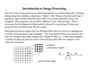
31. Modelisation Data acquisition system output input 50 50 100 100 150 150 200 200 250 250 50 100 150 200 250 50 100 150 200 250 image Real scene O = h * i + n noise distortions … Convolution  2D systems  mathematical tools  filtering

32. Chaîne de traitement Formation of the image (tomography, radar,…) Compression (lossless or lossy) TRANS- MISSION SENSOR Enhancement (histogram, colors,...) VISUALIZATION Restoration (filtering, deconvolution) Recognition (Automatic or supervised decisions) Segmentation (extraction of informations) AUTOMATIC PROCESSING

33. Applications • Remote sensing : satellites, aircraft, spacecraft • Image transmission, storage • medical • radar, sonar • acoustic • automated inspection of industrial parts • … Satellites : useful in tracking or earth ressources geographical mapping prediction of agricultural crop urban growth weather flood and fire control ... Thematicians  Scientifics

34. Examples of analysis tasks Equalization of histogram Image enhancement

35. Idem

36. Télécommunications TV numérique, Internet, Téléphonie, … • Compression d’images, cryptage, tatouage Image compressée Taux 1: 256 Image pleine précision Image compressée Taux 1: 64

37. Examples

40. Other examples

41. Imagerie spatiale Observation du ciel (astronomie) et de la Terre (télédétection) • compression, restauration, segmentation, reconnaissance Image du ciel, dans la bande U.V. Image Radar Image SPOT (optique)

42. Vision industrielle, robotique Contrôle industriel, biométrie • segmentation, reconnaissance Images infrarouges Répartition de chaleur

43. Imagerie médicale Diagnostic, imagerie fonctionnelle, télémédecine, biologie, ... • formation d’images, compression, restauration, segmentation, détection,... Coupe radiographique d’un crâne Image échographique d’un foetus

44. Défense, surveillance, sécurité Militaire, surveillance de site, ... • Compression, cryptage, restauration, segmentation, reconnaissance Poursuite d’avion sur image optronique

45. Global system Light f(t) Sensor f(x,y) (pre)processing matrix g(x,y) Bases of the world Base de relation Segmentation list E={ei} ei = {(xi,yj)} Classification Recognition Graph of objects Interpretation of the scene (chaînage arrière) Reseau semantique Operation Data structure

46. Hierarchy of processing • Low level • preprocessing, high data volume, low algorithmic complexity (filtering, FFT, …) • Medium level • feature extraction (segmentation) • High level • image understanding, low data volume, high algorithmic complexity Image processing Artificial intelligence (bases, rules)

47. Hierarchy of processing (2) • Generalised images • Segmented images • Geometric representation • Information models M flops Complexity LL HL LL HL Complexity depends on what the operator wants !

48. Example

49. Image Processing: • Image  Image • Computer Vision: • Image  Description • Computer Graphics: • Description  Image

50. Tools No algorithm is done here Softwares : Matlab, Khoros, …, C, Fortran... Computer+software result Data acquisition