Load Prediction for Best Effort Real Time

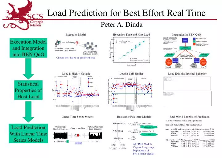
1. CMU load prediction software uses linear time series models to predict load on each host. • QuO delegate choses server replica based on load predictions • Integration by Peter A. Dinda • and Xiaoming Liu Application code ARFIMA(p,d,q) Client BBN QuO System Infinite # roots CMU Load Prediction (Peter A. Dinda) ARIMA(p,d,q) Delegate with Hysteresis d roots ARMA(p,q) LoadPred Syscond LoadPred Syscond Delegate chooses server replica based on load predictions Load Prediction Engine Server Replica Server Replica Load Prediction Engine AR(p) MA(q) Other Jobs Other Jobs Host A Host B ? [tmin,tmax] Interactive Application Short tasks with deadlines Unmodified COTS Distributed System Unpredictable Random Sequence Partially Predictable Load Sequence Fixed Linear Filter Load Prediction for Best Effort Real Time Peter A. Dinda Execution Model Execution Time and Host Load Integration In BBN QuO Execution Model and Integration into BBN QuO Choose host based on predicted load Load is Highly Variable Load is Self Similar Load Exhibits Epochal Behavior Statistical Properties of Host Load Linear Time Series Models Realizable Pole-zero Models Real World Benefits of Prediction sa is the confidence interval for t+1 predictions Map work that would take 100 ms at zero load axp0: sz=0.54, m=1.0, sa(ARMA(4,4))= 0.109 sa(ARFIMA(4,d,4))= 0.108 no model: 1.0 +/- 1.06 (95%) => 100 to 306 ms ARMA: 1.0 +/- 0.22 (95%) => 178 to 222 ms ARFIMA: 1.0 +/- 0.21 (95%) => 179 to 221 ms axp7: sz=0.14, m=0.12, sa(ARMA(4,4))= 0.041 sa(ARFIMA(4,d,4))= 0.025 no model: 0.12 +/- 0.27 (95%) => 100 to 139 ms ARMA: 0.12 +/- 0.08 (95%) => 104 to 120 ms ARFIMA: 0.12 +/- 0.05 (95%) => 107 to 117 ms Load Prediction With Linear Time Series Models ARFIMA Models Capture Long-range Dependence of Self-Similar Signals