Download
1 / 26
260 likes | 388 Views
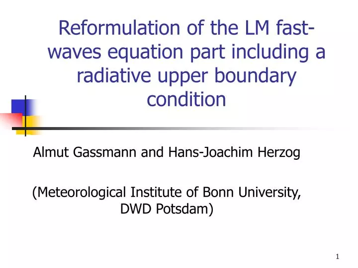
Reformulation of the LM fast-waves equation part including a radiative upper boundary condition. Almut Gassmann and Hans-Joachim Herzog (Meteorological Institute of Bonn University, DWD Potsdam). F(n). n. n*. n+1. F(n*). Short review…. Fast waves and slow tendencies

E N D
Reformulation of the LM fast-waves equation part including a radiative upper boundary condition Almut Gassmann and Hans-Joachim Herzog (Meteorological Institute of Bonn University, DWD Potsdam)
F(n) n n* n+1 F(n*) Short review… • Fast waves and slow tendencies • improper mode separation • improper combination in case of the Runge-Kutta-variants • Further numerical shortcomings • divergence damping • vertical implicit weights: symmetry: buoyancy term <-> other implicit terms • lower boundary condition • Time integration is divided into 2 parts • Fast waves (gravity and sound waves) • Slow tendencies (including advection)
2-time-level scheme (KW-RK2-short) Comments on the Murthy-Nanundiah-test (Baldauf 2004) The test relies on the equation whose stationary solution is known as f=g/b . Baldauf claimed that the KW-RK2-short-scheme was not suitable since the splitting into fast forcing and slow relaxation does not yield the correct stationary solution. BUT: The splitting into slow forcing and fast relaxation does. What is our approch alike? -> slow forcing and fast relaxation Forcing: physical and advective processes, nonlinear ones Relaxation: wave processes, linear ones
2-dimensional linear analysis of the fast wave part • Which is the state to • linearize around? • LM basic state (current) • or • State at timestep „n“, slow mode background Brunt-Vaisala-Frequency for the isothermal atmosphere Vertical advection of background pressure and temperature These terms are essential for wave propagation and energy consistency scale height variables are scaled to get rid of the density
Time scheme for fast waveshorizontal explicit – vertical implicit divergence damping symmetric implicitness (treatment as in other implicit terms) vertical temperature advection Remark: Acoustic and gravity waves are not neatly separable!
Divergence dampingRelative phase change With divergence damping Without divergence damping Phase speeds of gravity waves are distorted.
Symmetric implicitnessAmplification factor unsymmetric symmetric
Vertical advection of temperatureRelative phase change Without T-advection (nonisothermal atmosphere) With T-advection Phase speeds are incorrect. The impact in forecasts can hardly be estimated.
Conclusions from linear analysis • No divergence damping! • Symmetric implicit formulation! • Vertical temperature advection belongs to fast waves as well as vertical pressure advection! • Further conclusion: state to linearize around is state at time step „n“ and not the LM base state!
with for in vertical advection slow tendencies fast waves perturbation pressure or temperature Appropriate splitting
Lower boundary condition fast waves slow tendencies • „fast“ LBC • prescribe w(ke1) via • prescribe metrical term • in momentum equation via • (Almut Gassmann, COSMO • Newsletter 4, 2004, 155-158) „slow and fast“ LBC • prescribe Neumann boundary • conditions • with access to • which is also used to derive • surface pressure „slow“ LBC • prescribe • via • out of fast waves In that way we avoid any computational boundary condition.
Splitting slow modes and fast waves • Gassmann, Meteorol Atmos Phys (2004):“An improved two-time-level • split-explicit integration scheme for non-hydrostatic compressible models“ • Crank-Nicolson-method is used • for vertical advection. • Runge-Kutta-method RK3/2 is • used for horizontal advection only • and should not be mixed up with • the fast waves part. • Splitting errors of mixed methods (Wicker-Skamarock-type) are larger. • Gain of efficiency: • No mixing of slow-tendency computation with fast waves • No mixing of vertical advection with Runge-Kutta-steps
Mountain wave with RUBC w-field isothermal background and base state
Divergence and metric terms • Strong sensitvity of surface pressure at the lee side of the Alps, if different formulations of metric terms in the wind divergence are used • Conservation form (not used in the default LM version), • Direct control over in- and outflow across the edges • Alternative representation (used in the default LM version) u p u
Moisture profiles in Lindenberg with different LM-Versions (Thanks to Gerd Vogel) 7-day mean with oper. LM version and new version, dx=2.8 km
Conclusions and plans • Conclusions • The presented split-explicit algorithm is fully consistent and proven by linear analysis. • It needs no artificial assumptions and thus overcomes intuitive ad hoc methods. • Divergence formulation in terrain following is a very crucial point. • Plans • Higher order advection and completetion for more prognostic variables • Further realistic testing • Comparison with Lindenberg data