Download
1 / 24
250 likes | 378 Views
Lecture 3 Combinational Circuits. CSCE 211 Digital Design. Topics Basic Gates (3.1) Adders: half-adder, full-adder Gray Code (2.11) N-cube (2.14) Error Correcting codes (2.15) Boolean Algebra (4.1) Combinational-Circuit Analysis (4.2). August 28, 2003. Overview. Last Time

E N D
Lecture 3Combinational Circuits CSCE 211 Digital Design • Topics • Basic Gates (3.1) • Adders: half-adder, full-adder • Gray Code (2.11) • N-cube (2.14) • Error Correcting codes (2.15) • Boolean Algebra (4.1) • Combinational-Circuit Analysis (4.2) August 28, 2003
Overview • Last Time • Conversion of Fractions decimal base-r • Representations of Integers • Unsigned, signed magnitude, one’s complement, two’s complement • Arithmetic • BCD, representations of characters BCD, unicode • On last Time’s Slides(what we didn’t get to) • Basic gates (well almost on transparencies) • Adder circuits • New • Boolean algebra • Combinational circuits • VHDL • ButNot Table 4-36 page 277 • History: George Boole
Basic Gates • AND • OR • NOT
Basic Gates • NAND • NOR • XOR
Gray Code • In some mechanical devices you want to encode positions as binary strings in such a way that positions close to each other are represented by strings that are close together. • Gray code – adjacent position differ in only one bit • 000 • 001 • 011 • 010 • 110 • 111 • 101 • 100 • Figure 2-6 encoding disk
Construction of Gray Codes • Gray Codes are reflective • Algorithm for construction of Gray Codes on n-bits • A 1-bit Gray code has two words 0 and 1. • The first 2n words of an (n+1)-bit gray code are the words of the n-bit gray code with a leading 0 added. • The next 2n words of an (n+1)-bit gray code are the words of the n-bit gray code but written in reverse order with a leading 1 added.
Construction of Gray Codes 4-bit gray code • 0 000 • 1-bit gray code • 0 • 1 • 2-bit gray code • 00 • 01 • 11 • 10 • 3-bit gray code • 0 00 • 0 01 • 0 11 • 0 10 • 1 10 • 1 11 • 1 01 • 1 00
Gray Code Generation Algorithm 2 • Algorithm • The bits of an n-bit binary and n-bit Gray-code code word are numbered from right to left from 0 to n-1. • Bit i of a Gray-code word is 0 if bits i and i+1 of the corresponding binary code word are the same, else bit i is 1. (When i = n-1, bit n is considered to be 0.) • Example • Given 0100 1010 • Add fake 0 on front bit n is 0 • 0 0100 1010 0110 1111
Codes representing characters • ASCII (American Standard Code for Information Interchange) – 8 bits = 7 + parity • Unicode 16 bits
N-cubes • 1-cube • 2-cube • 3-cube • Traversing in gray-code order
Parity Bits • Even parity bit – parity bit is set so that the number of ones is even • Odd parity bit
Error Correcting codes • For an n-bit code, consider the hypercube of dimension n • Choose some subset of the nodes as code words. • Suppose the distance between any two two code words is at least 3. • Now consider transmission errors. • Then if there is an error in transmitting just one bit then the distance from the received word to one code word is one, distances to other code words are at least two. • Single error correcting, double error detecting. • Such codes are called Hamming codes after their inventor Richard Hamming.
Boolean Algebra • George Boole (1854) invented a two valued algebra • To “give expression … to the fundamental laws of reasoning in the symbolic language of a Calculus.” • 1938 Claude Shannon at Bell Labs noted that this Boolean logic could be used to describe switching circuits. (Switching Algebra) • In Shannon’s view a relay had two positions open and closed and collections of relays satisfied the properties of Boolean algebra.
Boolean Algebra Axioms • The axioms of a mathematical system are a minimal set of properties that are assumed to be true. • Axioms of Boolean Algebra • X = 0 if X != 1 X=1 if X!=0 • If X = 0, then X’ = 1 if X=1 then X’=0 • 0 . 0 = 0 1 + 1 = 1 • 1 . 1 = 1 0 + 0 = 0 • 0 . 1 = 1 . 0 = 0 1 + 0 = 0 + 1 = 1 • Axioms 1-5 and 1-5’ completely define Boolean algebra.
Boolean Algebra Theorems • Proofs by perfect induction
More Theorems • N.B. T8¢, T10, T11
Duality • Swap 0 & 1, AND & OR • Result: Theorems still true • Why? • Each axiom (A1-A5) has a dual (A1¢-A5¢) • Counterexample:X + X × Y = X (T9)X × X + Y = X (dual)X + Y = X (T3¢)???????????? X + (X×Y) = X (T9)X× (X + Y) = X (dual)(X× X) + (X× Y) = X (T8)X+ (X× Y) = X (T3¢) parentheses,operator precedence!
N-variable Theorems • Prove using finite induction • Most important: DeMorgan theorems
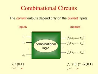
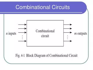
Combinational Circuit Analysis • A combinational circuit is one whose outputs are a function of its inputs and only its inputs. • These circuits can be analyzed using: • Truth tables • Algebraic equations • Logic diagrams