Download
1 / 51
510 likes | 744 Views
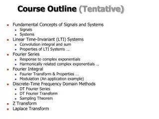
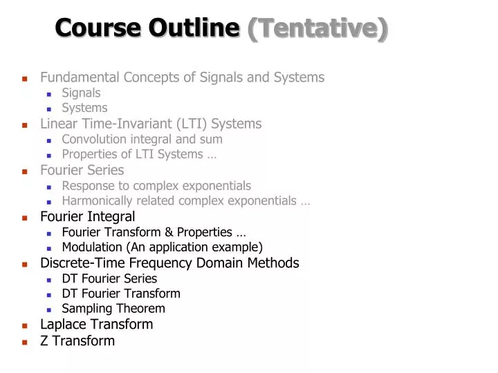
Course Outline (Tentative). Fundamental Concepts of Signals and Systems Signals Systems Linear Time-Invariant (LTI) Systems Convolution integral and sum Properties of LTI Systems … Fourier Series Response to complex exponentials Harmonically related complex exponentials …

E N D
Course Outline (Tentative) • Fundamental Concepts of Signals and Systems • Signals • Systems • Linear Time-Invariant (LTI) Systems • Convolution integral and sum • Properties of LTI Systems … • Fourier Series • Response to complex exponentials • Harmonically related complex exponentials … • Fourier Integral • Fourier Transform & Properties … • Modulation (An application example) • Discrete-Time Frequency Domain Methods • DT Fourier Series • DT Fourier Transform • Sampling Theorem • Laplace Transform • Z Transform
Continuous–Time Fourier Transform • So far, we have seen periodic signals and their representation in terms of linear combination of complex exponentials. • Practical meaning: • superposition of harmonically related complex exponentials. • How about aperiodic signals?
... ... Fourier Transform Representation of Aperiodic Signals • (An aperiodic signal is a periodic signal with infinite period.) • Let us consider continuous-time periodic square wave
Fourier Transform Representation of Aperiodic Signals • Recall that the FS coefficients are: • Let us look at it as:
Fourier Transform Representation of Aperiodic Signals as , closer samples, faster rate! as , periodic square wave rectangular pulse (aperiodic signal) , FS coefficients xT envelope itself Think of aperiodic signal as the limit of a periodic signal
Fourier Transform Representation of Aperiodic Signals Examine the limiting behaviour of FS representation of this signal Consider a signal that is of finite duration,
... ... t Fourier Transform Representation of Aperiodic Signals • We can construct a periodic signal out of with period • For FS representation of periodic signal
Fourier Transform Representation of Aperiodic Signals Since (Recall and envelope case) as the envelope of Define
Fourier Transform Representation of Aperiodic Signals Hence, : inverse Fourier transform Fourier Transform pair : Fourier transform (spectrum) information needed for describing x(t) as a linear combination of sinusoids
Dirichlet conditions guarantee that at any t except at discontinuities (similar to periodic case). i) x(t) is absolutely integrable, Convergence of Fourier Transform ii) x(t) has a fiinite number of maxima and minima within any finite interval iii) x(t) has a finite number of discontinuities within any finite interval. Further more each of these discontinuities must be finite.
x(t) t T1 -T1 X(ω) 2T1 ω Example
X(ω) ω -W W x(t) t Example (cont’d)
x(t) X(ω) ω t -W W T1 -T1 x(t) X(ω) 2T1 t ω Note Narrow in Time Domain have Broad FT! Broad in Time Domain Narrow FT! (Scaling property)
then Fourier Transform For Periodic Signals Consider a signal x(t) with Fourier Transform (i.e., a signal impulse of area 2 at ω=ω0) Let us find the signal if X(ω) is a linear combination of impulses equally spaced in frequency, i.e., : FS representation of periodic signal
Fourier Transform For Periodic Signals Hence, FT of periodic signal is weighted impulse train occuring at integer multiples of ω0 Example: a) Periodic square wave: Recall FS coefficients of periodic square wave (from previous chapter)
X(ω) -ω0 ω0 FT is again impulse train in frequency domain with period Fourier Transform For Periodic Signals b) x(t)=sinω0t x(t)=cosω0t c) impulse train
Properties of CT Fourier Transform Notations: 1.Linearity: Prove it as an exercise!
Properties of CT Fourier Transform 2.Time Shifting: Proof: F{x(t-t0)}
X(t) X1(t) X2(t) 1.5 1 1 1 t t t 1 2 3 4 Properties of CT Fourier TransformExample By linearity and time-shifting properties of FT
Properties of CT Fourier Transform 3.Conjugation / Conjugate Symmetry: for real x(t) Opp. pg. 303 forproof ! 4.Differentiation & Integration: Multiplication in frequency domain * Important in solving linear differential equations:
Properties of CT Fourier TransformExample Consider Take FT of both sides; For
Properties of CT Fourier TransformExample Consider (unit step) For
Properties of CT Fourier Transform 5.Time and Frequency Scaling: (Prove using FT integral) Remark: - Inverse relation between time and frequency domains: - A signal varying rapidly will have a transform occupying wider frequency band, and vice versa -
Properties of CT Fourier Transform 6.Duality: Observe the FT and inverse FT integrals: Recall Symmetry between the FT pairs! In general;
Properties of CT Fourier Transform Example: By duality; (prove it!) Dual of the properties: (frequency differentiation) (frequency shifting)
Properties of CT Fourier Transform 7.Parseval’s Relation: total energy in x(t) (Check the proof in Opp. pg.312) energy density spectrum
Properties of CT Fourier TransformConvolution Property (Additional & very important properties of FT, in terms of LTI systems) Take FT.
Properties of CT Fourier TransformConvolution Property Convolution of two signals in time domain is equivalent to multiplication of their spectrums in frequency domain frequency response of the system Example: a) Consider a CT, LTI system with Recall the time-shifting property of FT Frequency response is
H(ω) 1 ω -ωc 0 ωc stopband Passband stopband Properties of CT Fourier TransformConvolution Property b) Frequency-selective filtering: achieved by an LTI system whose frequency response H(ω) passes desired range of frequencies and stops (attenuates) other frequencies, e.g., ideal lowpass filter
S(ω) A ω -ω1 ω1 Properties of CT Fourier TransformMultiplication Property From convolution property and duality, multiplication in time domain corresponds to convolution in frequency domain. Amplitude Modulation (multiplication of two signals) important in telecommunications ! Example: Let s(t) has spectrum S(ω) Baseband signal
P(ω) ω -ω0 ω0 R(ω) -ω0-ω1 -ω0 -ω0+ω1 ω0-ω1 ω0 ω0+ω1 Properties of CT Fourier TransformMultiplication Property p(t)=cosω0t - Information (spectral content) in s(t) is preserved but shifted to higher frequencies (more suitable for transmission)
Properties of CT Fourier TransformMultiplication Property To recover: -Multiply r(t) with p(t)=cosω0t g(t)=r(t).p(t) -Apply lowpass filter!
Application of Fourier TheoryCommunication Systems Definitions: • Modulation: Embedding an info-bearing signal into a second signal. • Demodulation: Extracting the information bearing signal from the second signal. • Info-bearing signal x(t): The signal to be transmitted (modulating signal). • Carrier signal c(t): The signal which carries the info-bearing signal (usually a sinusoidal signal).
Application of Fourier TheoryCommunication Systems Modulated signaly(t) is then the product of x(t) and c(t) • individual voice signals are in 200Hz-4kHz y(t)=x(t).c(t) Objective: To produce a signal whose frequency range is suitable for transmission over communication channel. e.g.: • telephony (long-distance) over microwave or satellite links in 300MHz-300GHz (microwave), 300MHz-40GHz (satellite) Information in voice signals must be shifted into these higher ranges of frequency
Application of Fourier Theory Amplitude Modulation with Complex Exponential Carrier ωc: carrier frequency Consider θc=0 From multiplication property
X(ω) C(ω) 1 ω ω -ωm ωm ωc Y(ω) 1 ω ωc ωc+ ωm ωc- ωm Application of Fourier Theory Amplitude Modulation with Complex Exponential Carrier * To recover x(t) from y(t): (Shift the spectrum back) (Demodulation)
x(t) y(t) Y(ω) ω -ωc- ωm -ωc -ωc+ ωm ωc+ ωm ωc- ωm ωc Application of Fourier Theory Amplitude Modulation with Sinusoidal Carrier For θc=0 , y(t)=x(t)cosωct ,
X(ω) 1 -ωm ωm Application of Fourier Theory Amplitude Modulation with a Sinusoidal Carrier To recover x(t) from y(t), the condition ωc>ωm must be satisfied! Otherwise, the replicas will overlap. Example: Y(ω) 1 -ωm- ωc -ωc ωc ωm+ ωc
Application of Fourier Theory Demodulation for Sinusoidal Amplitude Modulation To recover the information-bearing signal x(t) at the receiver Synchronous Demodulation: Transmitter and receiver are synchronized in phase x(t) can be recovered by modulating y(t) with the same sinusoidal carrier and applying a lowpass filter. (need to get rid of the 2nd term in RHS)
Y(ω) ω -ωc ωc+ ωm ωc- ωm ωc C(ω) W(ω) H(ω) ω ωc -ωc ω 2ωc 2ωc -ωm ωm 2ωc- ωm Application of Fourier Theory Demodulation for Sinusoidal Amplitude Modulation Apply lowpass filter (H(ω)) with a gain of 2 and cutoff frequency (ωco) ωm<ωco<2ωc-ωm
H(ω) 2 w(t) x(t) y(t) -ωco ωco lowpass filter y(t) x(t) Application of Fourier Theory Demodulation for Sinusoidal Amplitude Modulation In general,
Application of Fourier Theory Demodulation for Sinusoidal Amplitude Modulation Assume that modulator and demodulator are not synchronized; θc : phase of modulator φc : phase of demodulator
Application of Fourier Theory Demodulation for Sinusoidal Amplitude Modulation When we apply lowpass filter output x(t) output 0 must be maintained over time requires synchronization
envelope y(t) t Application of Fourier Theory Demodulation for Sinusoidal Amplitude Modulation Asynchronous Demodulation: Avoids the need for synchronization between the modulator and demodulator If the message signal x(t) is positive, and carrier frequency ωc is much higher than ωm (the highest frequency in the modulating signal), then envelope of y(t) is a very close approximation to x(t)
y(t)=(A+x(t)) cosωct x(t) A + + C y(t) R w(t) – – Application of Fourier Theory Demodulation for Sinusoidal Amplitude Modulation Envelope Detector : to assure positivity add DC to message signal, i.e., x(t)+A > 0 x(t) vary slowly compared to ωc (to track envelope) half-wave rectifier! cos ωct Tradeoff : simpler demodulator, but requires transmission of redundancy (higher power)
Y(ω) -ωc ωc Application of Fourier Theory Single-Sideband (SSB) Sinusoidal Amplitude Modulation Forωmis the highest frequency in x(t), total bandwidth of theoriginal signal 2ωm. X(ω) 2ωm ωm With sinusoidal carrier: spectrum shifted toωcand -ωc twice bandwidth is required. 4ωm Redundancy in modulated signal! Solution: Use SSB modulation
X(ω) Y(ω) ωm -ωc ωc ωc +ωm uppersideband lower sideband lower sideband upper sideband YU(ω) -ωc ωc YL(ω) -ωc ωc Application of Fourier Theory Single-Sideband (SSB) Sinusoidal Amplitude Modulation (DSB) Spectrum with upper sidebands (SSB) Spectrum with lower sidebands (SSB)
H(ω) yU(t) y(t) YU(ω) -ωc ωc Y(ω) -ωc ωc -ωc ωc Application of Fourier Theory Single-Sideband (SSB) Sinusoidal Amplitude Modulation For upper sidebands: Apply y(t) to a sharp cutoff bandpass/highpass filter.